Dimensionality reduction and feature transformation with scikit-learn.
Dimensionality Reduction: Feature Transformation
Feature Transformation
- The problem of pre-propressing a set of features (m) to create a new feature set (n) while retaining as much information as possible
- Number of features m reduced to n where
- $$m < n$$
- Transformation operator P^T
- $$P^Tx$$
- Number of features m reduced to n where
Ad Hoc Query Problem: Google Search
- A lot of words
- Polysemy (a word with multiple meanings)
- Car
- Automobile
- First element in a cons cell in Lisp
- This would give
- False positives
- Car
- Synonomy (multiple words with the same meaning)
- False negatives
- Polysemy (a word with multiple meanings)
- We can combine words together for better indicators
- We can solve this using 3 kinds of algorithms
- Principal Components Analysis
- Independent Components Analysis
- We can solve this using 3 kinds of algorithms
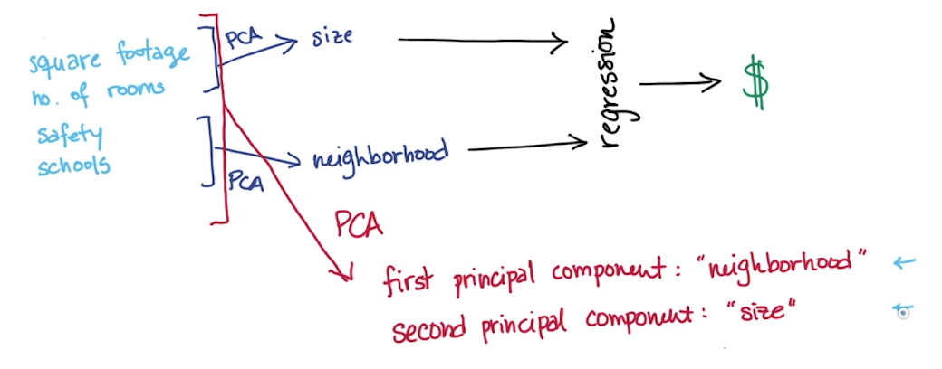
Measureable vs Latent Features
- Measurable features
- Square footage
- Number of rooms
- School ranking
- Neighborhood Safety
- Latent features: you're basically only "measuring" these 2 latent variables through all the measurable features
- Size
- Neighborhood
- How do we condense our features while preserving information?
- We can use Scikit-learn
- SelectKBest (k = no. of features to keep)
- In this scenario we should use this since we know we need only 2 latent variables
- This will throw all variables except the two which are the best
- SelectPercentile
- You could also use this and run at 50% for 2 features
- SelectKBest (k = no. of features to keep)
- We can use Scikit-learn
Principal Component
- We have many features, but we hypothesise a smaller number of features actually driving the patterns
- We can try making a composite feature (principle component) that more directly probes the underlying phenomenon
- Using PCA for dimensionality reduction
- Using PCA for unsupervised learning
- Example
- Measurable Features
- Square Footage
- Number of Rooms
- Latent Feature
- Size
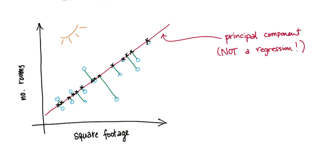
- We will project the points on the principle component
- It will be one dimension now
- Measurable Features
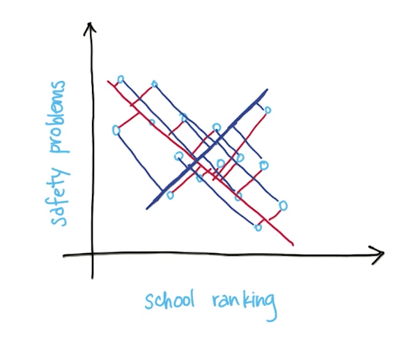
Determining the Principal Component
- Principal component of a dataset is the direction that has the largest variance
- Variance
- Spread of data distribution
- Retains the maximum amount of "information" in the original data
- Variance
Maximal Variance and Information Loss
- Information loss
- Example
- The length of the yellow line
- The longer the length, the more information loss
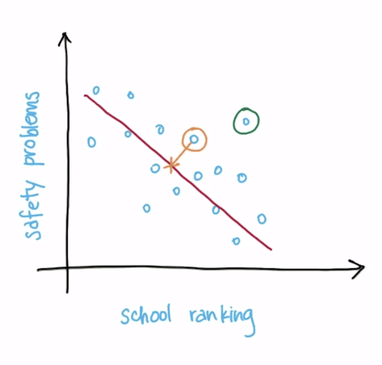
- Total information loss is the sum of all the projected distances from the points on the principal component
- Projection onto direction of maximal variance minimizes diatance from old (higher-dimensional) data point to its new transformed value
- Minimizes information loss (sum of red lines instead of blue lines)
- Example
Algorithm 1
PCA as a General Algorithm for Feature Transformation
When to use PCA
- Latent features driving the pattersn in data
- Dimensionality reduction
- Visualize high-dimensional data
- You can easily draw scatterplots with 2-dimensional data
- Reduce noise
- You get rid of noise by throwing away less useful components
- Make other algorithms work better with fewer inputs
- Very high dimensionality might result in overfitting or take up a lot of computing power (time
- A typical example is in eigenfaces
- You can use PCA to reduce the dimensionality to then use SVMs for example
- Visualize high-dimensional data
PCA Review
- Systematized way to transform input features into principal components (PC)
- Use PCs as new features
- PCs are directions in data that maximize variance (minimize information loss) when you project/compress donw onto them
- The more variance of data along a PC, the higher that PC is ranked
- Most variance, most information would be the first PC
- Second-most variance would be the second PC
- Max number of PCs = number of input features
PCA with Scikit-learn
In [10]:
# Import
from sklearn.decomposition import PCA
from sklearn import datasets
In [23]:
# Create data
iris = datasets.load_iris()
X = iris.data
y = iris.target
Standardizing
- Whether to standardize the data prior to a PCA on the covariance matrix depends on the measurement scales of the original features
- Since PCA yields a feature subspace that maximizes the variance along the axes, it makes sense to standardize the data, especially, if it was measured on different scales. Although, all features in the Iris dataset were measured in centimeters, let us continue with the transformation of the data onto unit scale (mean=0 and variance=1), which is a requirement for the optimal performance of many machine learning algorithms.
In [16]:
from sklearn.preprocessing import StandardScaler
X_std = StandardScaler().fit_transform(X)
In [19]:
# Instantiate
pca = PCA(n_components=2)

# Fit and Apply dimensionality reduction on X
pca.fit_transform(X_std)
Out[19]:
In [20]:
# Where the eigenvalues live
# You know first component and second component
# has a and b percent of the data respectively
pca.explained_variance_ratio_
Out[20]:
In [24]:
# Access components
pc_1 = pca.components_[0]
print(pc_1)
pc_2 = pca.components_[1]
print(pc_2)
PCA for Facial Recognition
- Facial recognition is good for PCA because
- Pictures of faces generally have high input dimensionality
- Many pixels
- Faces have general patterns that could be captured in smaller number of dimensions
- A pair of eyes
- Mouth
- Chin
- Pictures of faces generally have high input dimensionality
Scikit-learn: PCA for Facial Recognition
- We will be reducing 1850 PCs to 150 PCs
In [86]:
from time import time
import logging
import pylab as pl
from sklearn.cross_validation import train_test_split
from sklearn.datasets import fetch_lfw_people
from sklearn.grid_search import GridSearchCV
from sklearn.metrics import classification_report, confusion_matrix, f1_score
from sklearn.decomposition import RandomizedPCA
from sklearn.svm import SVC
In [68]:
# Data of famous people's faces
faces = fetch_lfw_people(min_faces_per_person=70, resize=0.4)
X = faces.data
y = faces.target
target_names = faces.target_names
n_classes = target_names.shape[0]

# Split data
X_train, X_test, y_train, y_test = train_test_split(X, y, test_size=0.25, random_state=42)
In [78]:
# Introspect the images arrays to find the shapes (for plotting)
n_samples, h, w = faces.images.shape

# For machine learning we use the data directly (as relative pixel
# position info is ignored by this model)
X = faces.data
n_features = X.shape[1]

# the label to predict is the id of the person
y = faces.target
target_names = faces.target_names
n_classes = target_names.shape[0]

print("Total dataset size:")
print("n_samples: %d" % n_samples)
print("n_features: %d" % n_features)
print("n_classes: %d" % n_classes)
In [65]:
# Compute a PCA (eigenfaces) on the face dataset
n_components = 150

print("Extracting the top {} eigenfaces from {} faces".format(n_components, X_train.shape[0]))
pca = RandomizedPCA(n_components=n_components, whiten=True).fit(X_train)

# eigenfaces: principal components
# Takes pca.components and reshape them
# We've gone from 1800 to 150
eigenfaces = pca.components_.reshape((n_components, h, w))

# Transform data into principal components representation
print("Projecting the input data on the eigenfaces orthonormal basis")
X_train_pca = pca.transform(X_train)
X_test_pca = pca.transform(X_test)
In [62]:
# Train an SVM classification model

print("Fitting the classifier to the training set")

param_grid = {
    'C': [1e3, 5e3, 5e4, 1e5],
    'gamma':[0.0001, 0.0005, 0.001, 0.005, 0.01, 0.1]
}

# Instantiate model
svm = SVC(kernel='rbf', class_weight='balanced', random_state=42)

# GridSearch
clf = GridSearchCV(svm, param_grid)
clf.fit(X_train_pca, y_train)
print(clf.best_estimator_)
In [76]:
# Quantitative evaluation of the model quality on the test set
print("Predicting the people names on the testing test")
y_pred = clf.predict(X_test_pca)
In [74]:
# Classification report and confusion matrix
print(classification_report(y_test, y_pred, target_names=target_names))
In [92]:
# F1-score average
# The F1 score can be interpreted as a weighted average of the precision and recall
# Where an F1 score reaches its best value at 1 and worst score at 0
# The relative contribution of precision and recall to the F1 score are equal
# The formula for the F1 score is:
# F1 = 2 * (precision * recall) / (precision + recall)

print(f1_score(y_test, y_pred, average='weighted'))
In [79]:
# Confusion Matrix
print(confusion_matrix(y_test, y_pred, labels=range(n_classes)))
In [82]:
# Qualitative evaluation of the predictions using matplotlib
%matplotlib inline

def plot_gallery(images, titles, h, w, n_row=3, n_col=4):
    """Helper function to plot a gallery of portraits"""
    pl.figure(figsize=(1.8 * n_col, 2.4 * n_row))
    pl.subplots_adjust(bottom=0, left=.01, right=.99, top=.90, hspace=.35)
    for i in range(n_row * n_col):
        pl.subplot(n_row, n_col, i + 1)
        pl.imshow(images[i].reshape((h, w)), cmap=pl.cm.gray)
        pl.title(titles[i], size=12)
        pl.xticks(())
        pl.yticks(())


# plot the result of the prediction on a portion of the test set

def title(y_pred, y_test, target_names, i):
    pred_name = target_names[y_pred[i]].rsplit(' ', 1)[-1]
    true_name = target_names[y_test[i]].rsplit(' ', 1)[-1]
    return 'predicted: %s\ntrue:      %s' % (pred_name, true_name)

prediction_titles = [title(y_pred, y_test, target_names, i)
                         for i in range(y_pred.shape[0])]

plot_gallery(X_test, prediction_titles, h, w)

# plot the gallery of the most significative eigenfaces

eigenface_titles = ["eigenface %d" % i for i in range(eigenfaces.shape[0])]
plot_gallery(eigenfaces, eigenface_titles, h, w)

pl.show()


Variance explained by each principal component
In [85]:
# Variance explained by first component: 0.19346474
# Variance explained by second component: 0.15116931
pca.explained_variance_ratio_
Out[85]:
F1 score variation as we change the number of principal components
- How do we select how many PCs to use?
- Train on different number of PCs
- See how accuracy responds
- Cut off when it becomes apparent that adding more PCs doe not buy you much more discrimination
- DO NOT select features before performing PCA
- Train on different number of PCs
- As you add more PCs
- It should give you additional signal to improve our performance
- But it is also possible that we end up with greater complexity resulting in overfitting
In [100]:
PC = [10, 15, 25, 50, 100, 250]
scores = []

for i in PC:
    # Loop through number of components
    n_components = i

    # Instantiate
    pca = RandomizedPCA(n_components=n_components, whiten=True).fit(X_train)

    # Redefine training data
    X_train_pca = pca.transform(X_train)
    X_test_pca = pca.transform(X_test)

    # Set param_grid
    param_grid = {
        'C': [1e3, 5e3, 5e4, 1e5],
        'gamma':[0.0001, 0.0005, 0.001, 0.005, 0.01, 0.1]
    }

    # Instantiate model
    svm = SVC(kernel='rbf', class_weight='balanced', random_state=42)

    # GridSearch
    clf = GridSearchCV(svm, param_grid, n_jobs=-1)
    clf.fit(X_train_pca, y_train)
    # clf.best_estimator_

    # Predict
    y_pred = clf.predict(X_test_pca)

    # Score
    score = f1_score(y_test, y_pred, average='weighted')

    # Append score to list
    scores.append(score)

print(scores)
In [103]:
# Zip the data to compare
list(zip(scores, PC))

# As you can see, the greater the number of PCAs, the greater the F1 score
# However, it starts to decrease when you have too many PCs
# You can see the decrease in f1_score from PCs=100 to PCs=250
Out[103]:
Algorithm 2
Independent Components Analysis (ICA)
- PCA
- Minimizing correlation by maximizing variance
- Cares about orthogonality
- Means that a relatively small set of primitive constructs can be combined in a relatively small number of ways to build the control and data structures of the language
- Finding "common characteristics"
- Eigenfaces problem
- ICA
- Finding independence by converting (through a linear transformation) your input features into a new feature space such that
- New features are independent of one another
- Cocktail party problem
- Mixed up sounds from each of the microphones
- Once you use an ICA algorithm, you can split the 3 sources into 3 independent features instead of the original sources with each source having a mix of everything
- Police car
- Foreign language
- News
- Finding independence by converting (through a linear transformation) your input features into a new feature space such that
| Property | PCA | ICA |
|---|---|---|
| Mutually Orthoganal | ✓ | |
| Mutually Independent | ✓ | |
| Maximal Variance | ✓ | |
| Maximal Mutual Information | ✓ | |
| Ordered Features | ✓ | |
| Bag of Features | ✓ | ✓ |
| Blind Source Separation Problem | ✓ | |
| Directional | ✓ |
ICA with Scikit-learn: Blind Source Separation
Other alternatives
- Random Components Analysis (RCA)
- Generates random directions (projections)
- Advantage over PCA and ICA
- Fast
- Simple
- Linear Discriminant Analysis (LDA)
- Finds a projection that discriminates based on the label