This is a short introduction to Octave for Machine Learning.
1. Basic Operations
- Not equal to
1 ~= 2
- And
1 && 2
- Or
1 || 2
- Variable
a = pi- 3.1316
- Print 2 decimal places
disp(sprintf('2 decimals: %0.2f', a))disp(sprintf('6 decimals: %0.6f', a))
- Longer decimal places
format shorta
- Matrices
- 3 x 2
A = [1 2; 3 4; 5 6]- Semicolon implies go to the next row
- 1 x 3
B = [1 2 3]
- 3 x 1
C = [1; 2; 3]
- 2 x 3 ones
ones(2, 3)D = 2*ones(2,3)
- 1 x 3 zeros
zeros(1, 3)
- 1 x 3 rand
rand(1, 3)
- 1 x 3 Gaussian Distribution, mean = 0, SD = 1
randn(1, 3)
- 3 x 2
- Start from 1, increment 0.1, up to 2
v = 1:0.1:2
- Start from 1, increment 1, up to 6
v = 1:6
- Histogram
w = -6 + sqrt(10)*(randn(1, 10))hist(w)- 50 bins
hist(w, 50)
- Identity Matrix
eye(4)- 4 x 4
eye(3)- 3 x 3
- quit
- press ‘q’
2. Moving Data Around
A = [1 2; 3 4; 5 6]- Getting matrix dimensions
size(A)- get first and second dimension
size(A, 1)size(A, 2)
- Get longest dimension (normally applied to vectors)
length(A)
- Load file
load file.dat
- Show variables in current workspace
who- for a more detailed version
whos
- Get data from file priceY
v = priceY(1:10)
- Save file
save hello.txt v -ascii;
- Accessing elements in matrix (array)
A(3, 2)- This would give row 6, column 2, so 6
A(2, :)- This would give all of row 2
A(:, 2)- This would give all of column 2
A([1,3], :)- This gives everything from Row 1, 3 and all Columns
- Replace Elements
A(:, 2) = [10; 11; 12]- This would replace second column (all rows)
- Append Elements
A = [A, [100; 101; 102]];- Appends new column vector [100; 101; 102]
- Put all elements of A into a single vector
A(:)
- Concatenate Matrices Horizontally
A = [1 2; 3 4; 5 6]B = [4 5; 6 7; 8 9]C = [A B]
- Concatenate Matrices Vertically
C = [A; B]
3. Computing on Data
A = [1 2; 3 4; 5 6]B = [11 12; 13 14; 15 16]C = [1 1; 2 2]- Muliply matrices
A*C
- Element-wise Multiplication
- Literal multiplication of cell to cell
- `[1 2] .* [2 2]
= [2 4]
- Element-wise squaring
A .^ 2- Squares each cell
- Element-wise reciprocal
1 ./ A
- Element-wise log and exponential
log(A)exp(A)
- Element-wise absolute value
abs(A)
- Add numbers to each cell
A + 1
- Transpose (m x n to n x m)
A'
- Maximum Value of matrix
max(A)- Does column-wise maximum
- Comparison
A < 3- 1: true
- 0: false
- Finding elements that fulfil inequality (vector)
find(A<3)- gives which elements are < 3
- Magic(num)
- Each row, column and diagonal add up to the same thing
- Something like sudoku
magic(3)
- Find which element in an array fulfills inequality
[r, c] = find(A >= 7)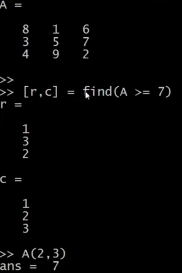
- Sum all elements
sum(A)
- Product all elements
prod(A)
- Round down
floor(A)
- Round up
ceil(A)
- Create random matrix
rand(3)max(rand(3), rand(3))- This takes max of 2 3x3 matrices
- Finding max per column
max(A, [], 1)
- Finding max per row
max(A, [], 2)
- Finding max of all numbers
max(max(A))
- Converting to vector
A(:)
- Sum each column
sum(A, 1)
- Sum each row
sum(A, 2)
- Sum diagonal
A .* eye(9)- Assuming A is 9 x 9
sum(sum(A .* eye(9)))sum(sum(A .* flipud(eye(9))))
- Inverse Matrix
pinv(A)
4. Plotting Data
t = [0:0.01:0.98];y1 = sin(2*pi*4*t);plot(t, y1);hold on;- This ‘hold on’ allows you to print two graphs together
y2 = cos(2*pi*4*t);plot(t, y2);xlabel('time')ylabel('value')legend('sin', 'cos')title('my plot')rint -dpng 'myPlot.png'- Save file
close- Get rid of figure
figure(1); plot(t, y1)figure(2); plot(t, y2)- Multiple figures
subplot(1, 2, 1);plot(t, y1);- Divides plot a 1 x 2 grid, access first element
subplot(1, 2, 2);plot(t, y2);- Divides plot a 1 x 2 grid, access second element
axis([0.5 1 -1 1])- x-axis: 0.5 to 1
- y-axis: -1 to 1
clf- Clear figure
imagesc(A), colorbar, colormap gray- Three commands using comma to chain commands
- Determine concentration of numbers on a grid
5. Control Statements
- for
- while
- else
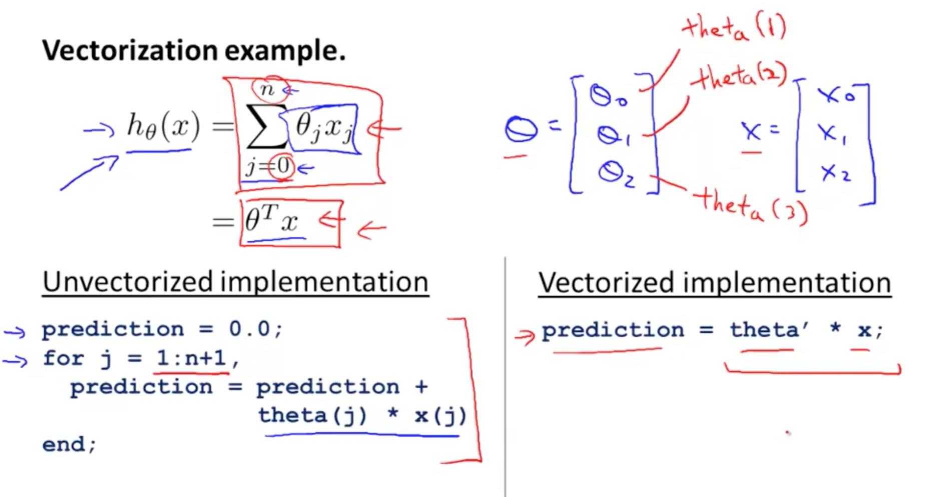
6. Vectorization
- Matlab/Octave index starts from 1
- Transposing theta would have a more simpler and efficient code
- Implementation in Octave
- Compress for loop to one line of vectorized code
- Vectorized implementation of gradient descent
- Delta and Theta are vectors
- Elements of Delta Vector (black boxes)
- Elements of Theta Vector (Theta0, Theta1, Theta2)
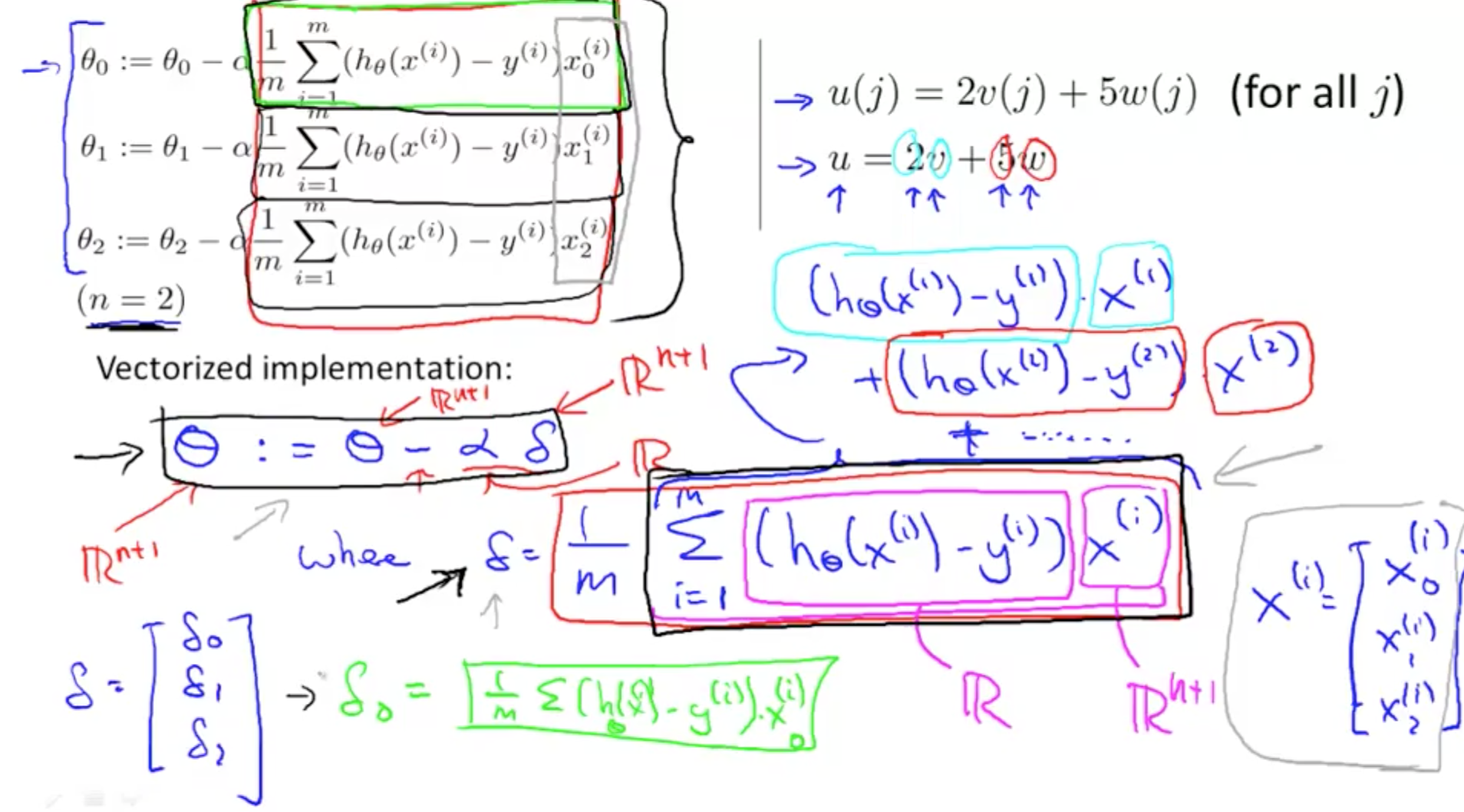
- Delta and Theta are vectors
Credits
I would like to give full credits to the respective authors as these are my personal python notebooks taken from deep learning courses from Andrew Ng, Data School and Udemy :) This is a simple python notebook hosted generously through Github Pages that is on my main personal notes repository on https://github.com/ritchieng/ritchieng.github.io. They are meant for my personal review but I have open-source my repository of personal notes as a lot of people found it useful.