Gaussian naive bayes, bayesian learning, and bayesian networks
Naive Bayes Methods
Bayes Rule: Intuitive Explanation
- (Prior probability)(Test evidence) --> (Posterior probability)
- Example
- P(C) = 0.01
- 90% it is positive if you have C (Sensitivity)
- 90% it is negative if you don't have C (Specificity)
- prior
- P(C) = 0.01
- P(C') = 0.99
- P(Pos|C) = 0.9
- P(Pos|C') = 0.1
- P(Neg|C') = 0.9
- P(Neg|C) = 0.1
- joint
- P(C and Pos) = P(C)P(Pos|C) = (0.01)(0.9) = 0.009
- P(C'and Pos) = P(C')P(Pos|C') = (0.99)(0.1) = 0.099
- normalizer
- P(Pos) = P(C and Pos) + P(C' and Pos) = 0.108
- posterior
- P(C|Pos) = 0.009 / 0.108 = 0.0833
- P(C'|Pos) = 0.099 / 0.108 = 0.9167
- Adding both = 1.0
- prior
Bayes Rule: Example
- This is really good for text learning
- Example
- P(Chris) = 0.5
- P(Love|Chris) = 0.1
- P(Deal|Chris) = 0.8
- P(Life|Chris) = 0.1
- P(Sara) = 0.5
- P(Love|Sara) = 0.5
- P(Love|Deal) = 0.2
- P(Love|Life) = 0.3
- P(Chris) = 0.5
In [40]:
p_chris_and_love_deal = 0.1*0.8*0.5

p_sara_and_love_deal = 0.5*0.2*0.5

normalizer = p_chris_and_love_deal + p_sara_and_love_deal

p_chris_given_love_deal = p_chris_and_love_deal / normalizer
p_sara_given_love_deal = p_sara_and_love_deal / normalizer

# P(Chris | "Love Deal")
print(p_chris_given_love_deal)

# P(Sara | "Love Deal")
print(p_sara_given_love_deal)
Bayes Rule: Theory
- Learn the best hypothesis given data and some domain knowledge
- Learn the most probable hypothesis given data and domain knowledge
- $$\underset{h∈H}{\mathrm{argmax}}P(h|D)$$
- h: some hypothesis
- D: some data
- argmax h∈H
- We want to maximize P(h|D)
- Bayes rule
- $$P(h|D) = \frac{P(D|h)P(h)}{P(D)}$$
- $$P(a,b) = P(a|b)P(b)$$
- $$P(a,b) = P(b|a)P(a)$$
- P(a,b) is the probability of a and b
- P(D)
- This is a normalizing term
- Prior on the data
- P(D|h)
- Data given the hypothesis
- $$D =\{x_i, d_i\}$$
- Training data, D, with inputs (x) and labels (d)
- What's the likelihood that given all of x_i and P(D|h) hypothesis is true, we will observe d's
- P(h)
- Prior on h
- Domain knowledge
- Say if you use KNN, you believe points close together would give similar outputs with higher likelihood than those far from one another
- $$P(h|D) = \frac{P(D|h)P(h)}{P(D)}$$
Bayesian Learning Algorithm
- For each h∈H, calculate P(h|D) ≈ P(D|h)
- Output
- $$h_1 = \underset{h}{\mathrm{argmax}}P(h|D)$$
- h_1: Maximum a posteriori
- $$h_2 = \underset{h}{\mathrm{argmax}}P(D|h)$$
- h_2: Maximum likelihood
- We're assuming P(h) and P(D) are uniform
- They're constants so we can ignore
- $$h_1 = \underset{h}{\mathrm{argmax}}P(h|D)$$
- Output
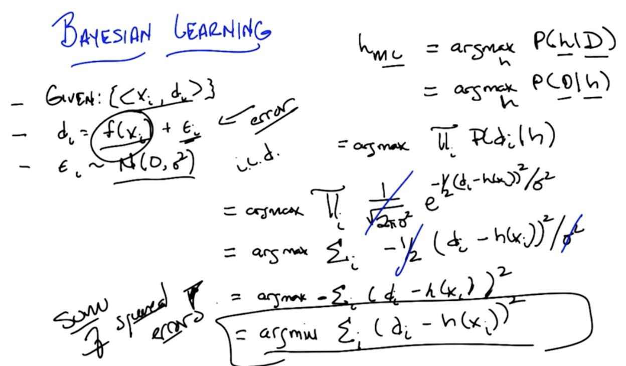
Gaussian Naive Bayes
- Ultimately we've simplified, using Gaussian distribution, to minimizing the sum of squared errors!
- Based on bayes rule we've ended up deriving sum of squared error
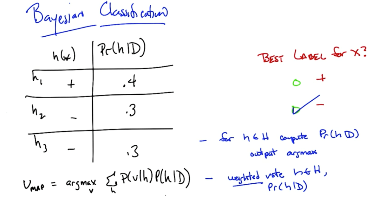
Bayesian Classification
- The algorithm changes slightly here
- We are maximizing the weighted vote instead of simply P(h|D)
Version Space
- The version space is a subset of the hypothesis space, where the hypotehesis space is a space of all possible hypotheses
- The version space are those hypotheses such that they correctly predict the training data you have (essentially a 100% model fit)
Bayesian Networks, Bayesian Nets, Belief Networks or Graphical Models
- Representing and dealing with probabilities
- Conditional independence
- X is conditionally independent of Y given Z if the probability distribution governing X is independent of the value of y given the value of Z
- P(X=x | Y=y, Z=z) = P(X=x | Z=z)
- More compactly
- P(X|Y,Z) = P(X|Z)
- X is conditionally independent of Y given Z if the probability distribution governing X is independent of the value of y given the value of Z
- Order of graph must be topological
- Graph must be acylic
- No cycles
- Graph must be acylic
- Sampling
- Two things distributions are for
- Probability of value
- Generate values
- Reasons for sampling
- Simulation of a complex process
- Approximate inference
- For machines
- We can't find the exact values because it may be hard and slower
- Visualization
- For humans to get a feel
- Two things distributions are for
- Inferencing Rules
- Marginalization
- $$P(x) = \underset{y}\sum(x,y)$$
- Chain rule
- $$P(x,y) = P(y|x)P(x) = P(y|x)P(y)$$
- Bayes rule
- $$P(y|x) = \frac {P(x|y)P(y)}{P(x)}$$
- Marginalization
Naive Bayes
- Say you've label A and B (hidden)
- Label A
- Have multiple words with different probabilities
- Every word gives evidence if it's label A
- We mutiply all the probabilities with the prior to find the joint probability of A
- Label B
- Have multiple words with different probabilities
- Every word gives evidence if it's label B
- We multiply all the probabilities with the prior to find the joint probability of B
- Now you can find out the probability of it being A or B
- Label A
- Reason why it's called Naive
- It ignores word order!
Naive Bayes Benefits
- Inference is cheap
- Linear
- Few parameters
- Estimate parameters with labeled data
- Connects inference and classification
- Empirically successful
Naive Bayes Training
- In the training process of a Bayes calssification problem, the sample data does the following:
- Estimate likelihood distributions of X for each value of Y
- Estimate prior probability P(Y=j)
Gaussian Naive Bayes in Scikit-learn
In [26]:
from sklearn.naive_bayes import GaussianNB
from sklearn.datasets import load_iris
from sklearn.cross_validation import train_test_split
from sklearn.metrics import accuracy_score
In [27]:
# Create features' DataFrame and response Series
iris = load_iris()
X = iris.data
y = iris.target

X_train, X_test, y_train, y_test = train_test_split(X, y, random_state=6)
In [28]:
# Instantiate: create object
gnb = GaussianNB()

# Fit
gnb.fit(X_train, y_train)

# Predict
y_pred = gnb.predict(X_test)

# Accuracy
acc = accuracy_score(y_test, y_pred)
acc
Out[28]: