Machine Learning theory and applications using Octave or Python.
1. Large Margin Classification
I would like to give full credits to the respective authors as these are my personal python notebooks taken from deep learning courses from Andrew Ng, Data School and Udemy :) This is a simple python notebook hosted generously through Github Pages that is on my main personal notes repository on https://github.com/ritchieng/ritchieng.github.io. They are meant for my personal review but I have open-source my repository of personal notes as a lot of people found it useful.
1a. Optimization Objective
- So far we have seen mainly 2 algorithms, logistic regression and neural networks. There are more important aspects of machine learning:
- The amount of training data
- Skill of applying the algorithms
- The SVM sometimes give a cleaner and more powerful way to learn parameters
- This is the last supervised learning algorithm in this introduction to machine learning
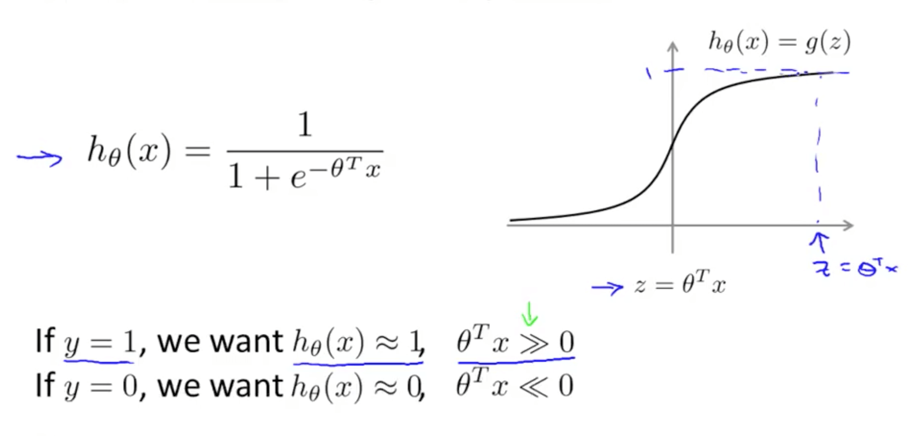
- Alternative view of logistic regression
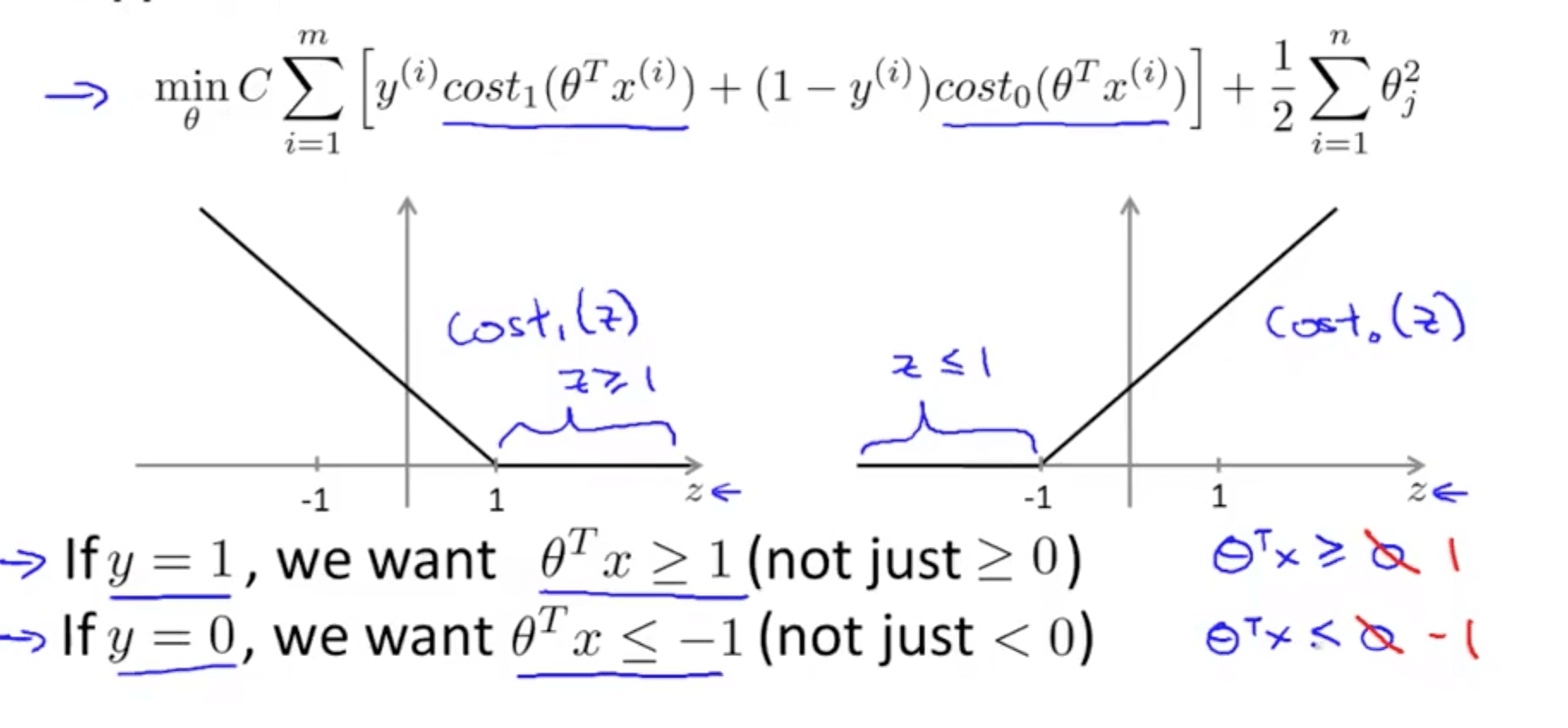
- If we want hθ = 1, we need z » 0
- If we want hθ = 0, we need z « 0
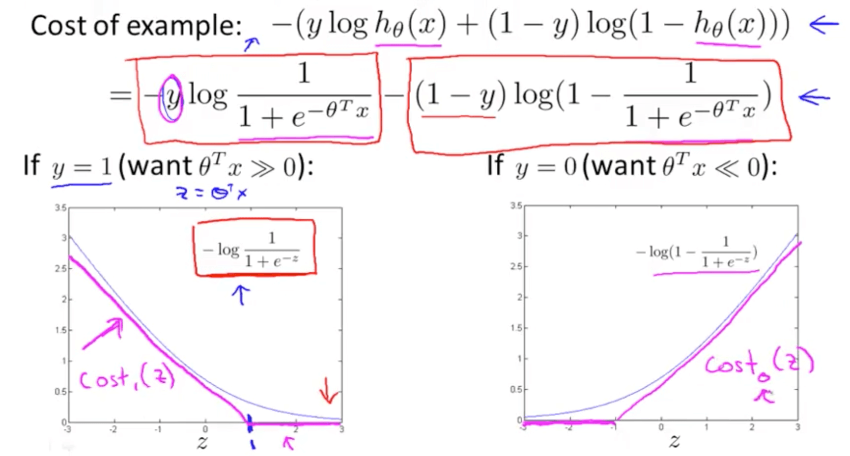
- If y = 1, only the first term would matter
- Graph on the left
- When z is large, cost function would be small
- Magenta curve is a close approximation of the log cost function
- If y = 0, only the second term would matter
- Magenta curve is a close approximation of the log cost function
- Diagram of cost contributions (y-axis)
- Support Vector Machine
- Changes to logistic regression equation
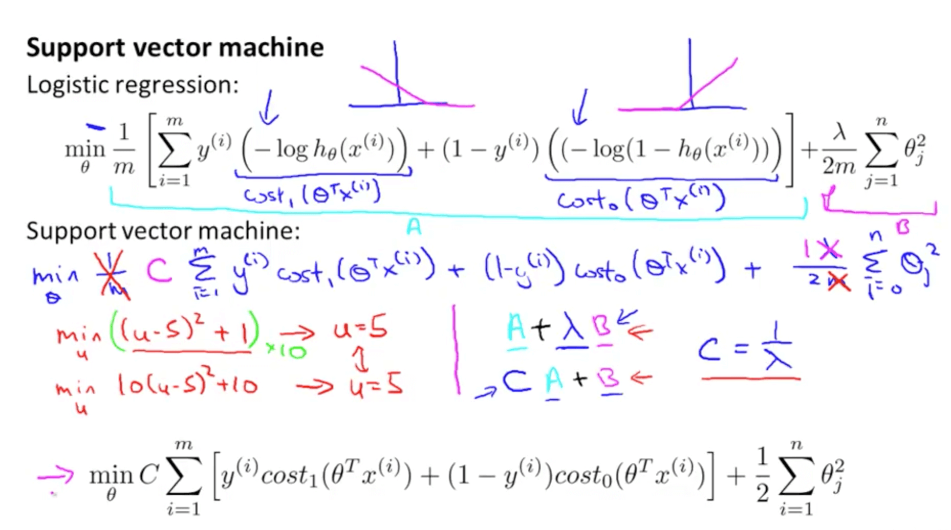
- We replace the first and second terms of logistic regression with the respective cost functions
- We remove (1 / m) because it does not matter
- Instead of A + λB, we use CA + B
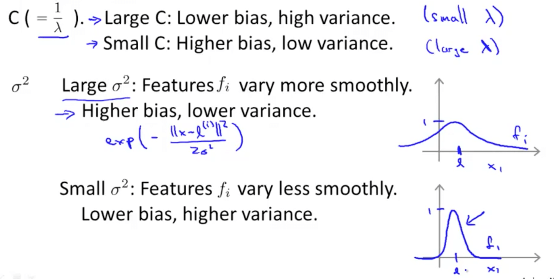
- Parameter C similar to the role (1 / λ)
- When C = (1 / λ), the two optimization equations would give same parameters θ
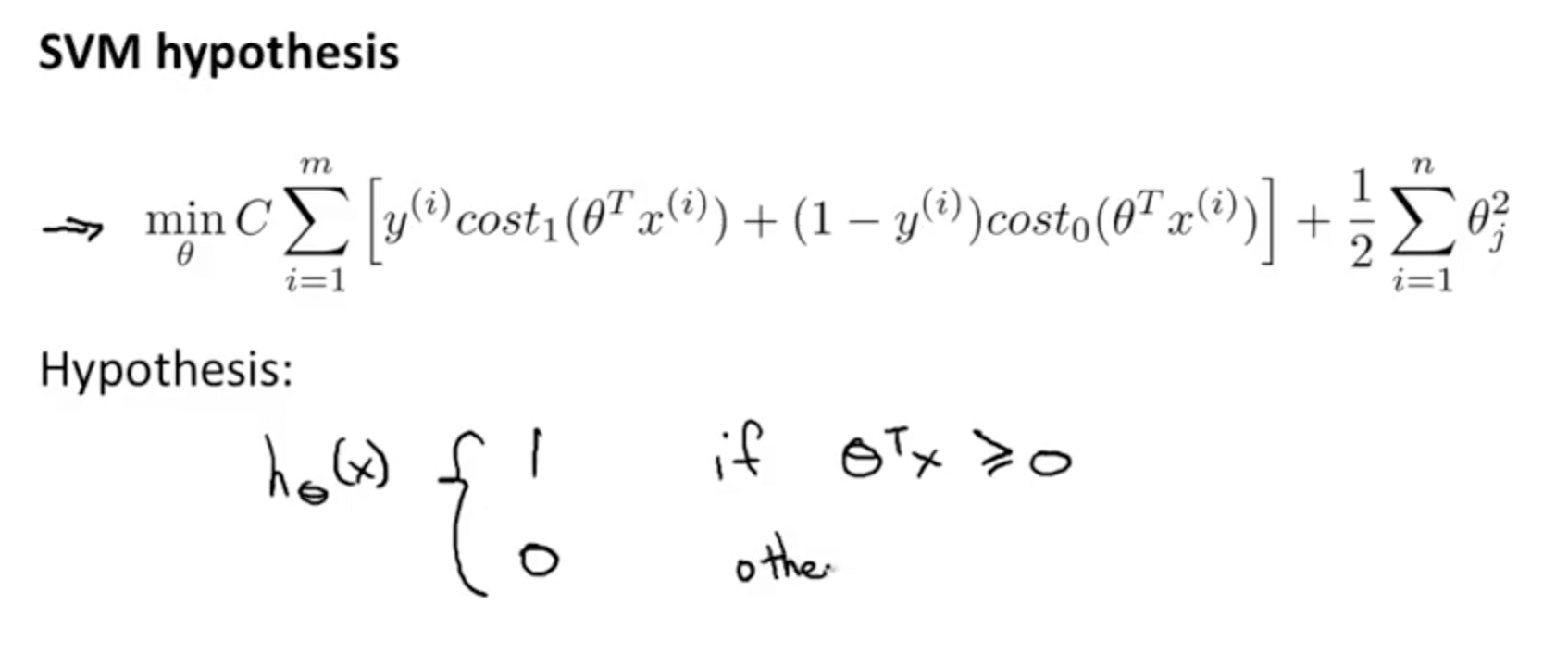
- Changes to logistic regression equation
- Compared to logistic regression, it does not output a probability
- We get a direct prediction of 1 or 0 instead
- If θTx is => 0
- hθ(x) = 1
- If θTx is <= 0
- hθ(x) = 0
- hθ(x) = 0
- If θTx is => 0
- We get a direct prediction of 1 or 0 instead
1b. Large Margin Intuition
- Some times people call Support Vector Machines “Large Margin Classifiers”
- SVM decision boundary
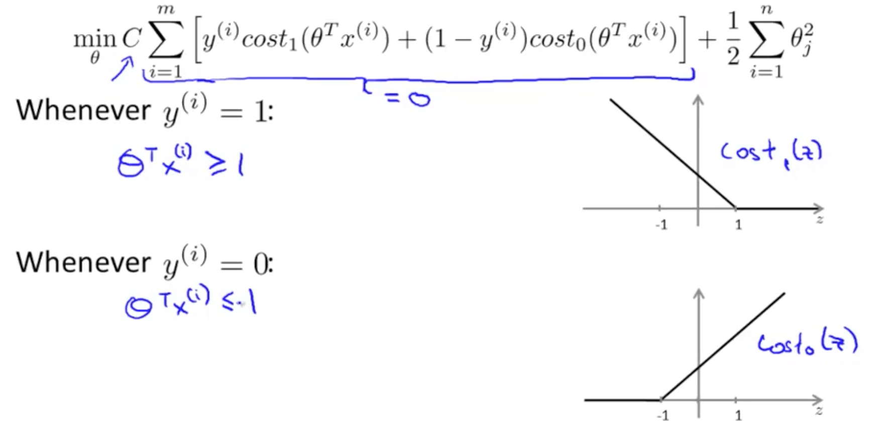
- If C is huge, we would want A = 0 to minimize the cost function
- How do we make A = 0
- If y = 1
- A = 0 such that θTx >= 1
- If y = 0
- A = 0 such that θTx <= -1
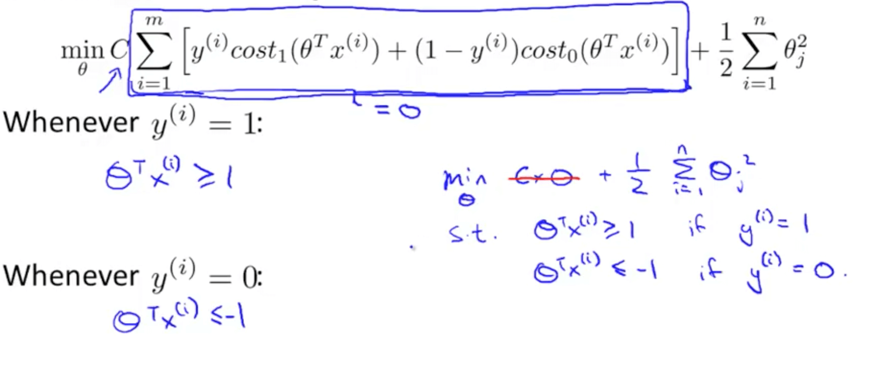
- If y = 1
- Since we want to ensure A = 0, our optimization problem boils down to minimizing the later term only
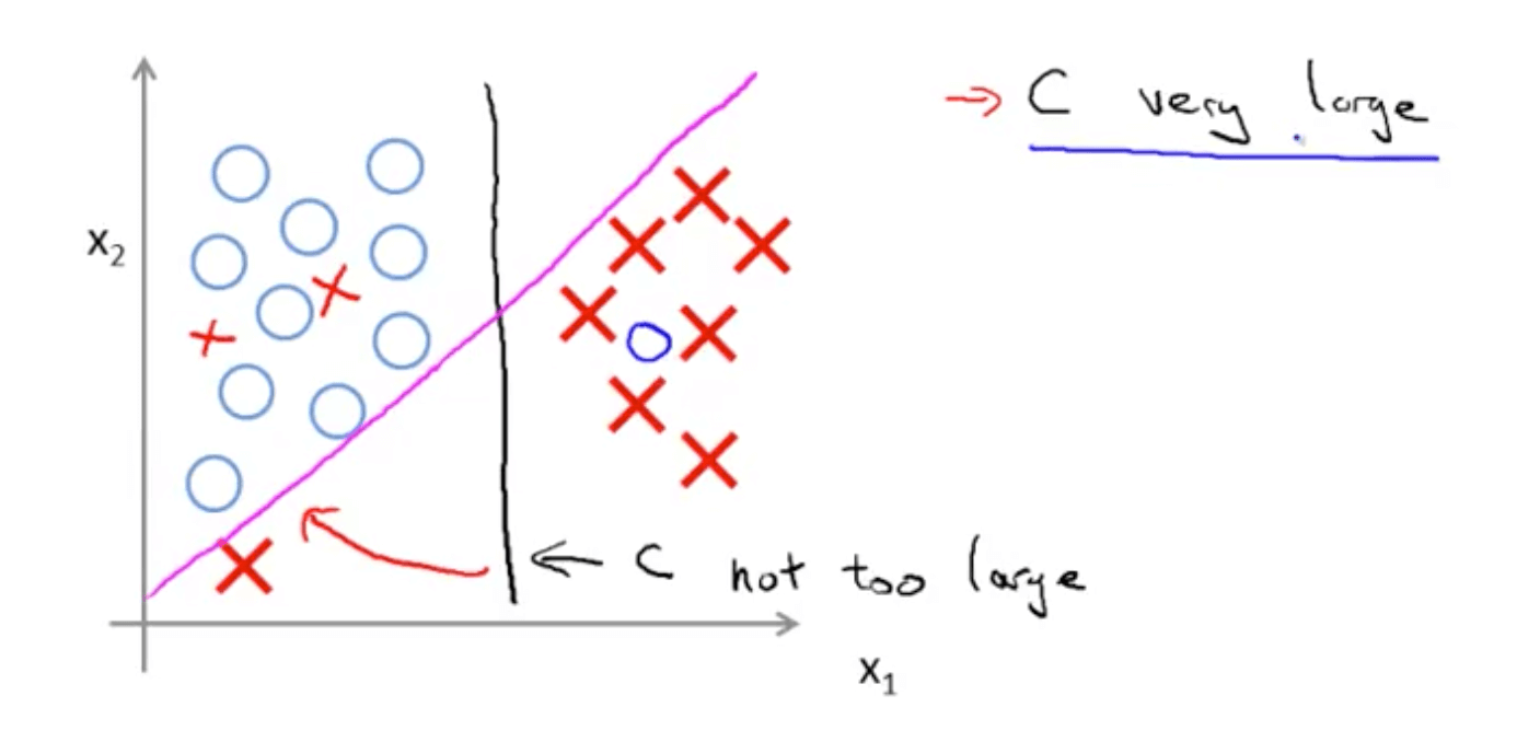
- SVM decision boundary: linearly separable case
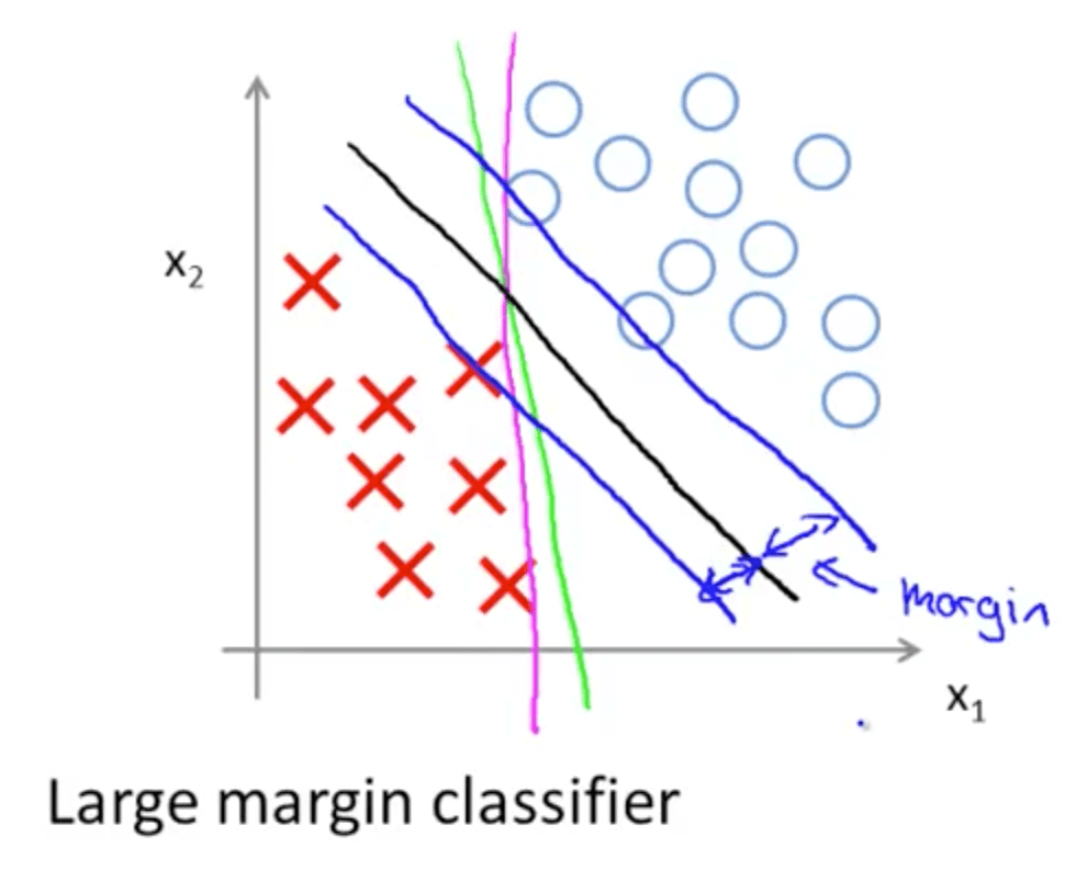
- Black decision boundary
- There is a larger minimum difference
- Chosen by SVM because of the large margins between the line and the examples
- Magenta and green boundaries
- Close to examples
- Distance between blue and black line: margin
- If C is very large
- Decision boundary would change from black to magenta line
- If C is not very large
- Decision boundary would be the black line
- SVM being a large margin classifier is only relevant when you have no outliers
- Black decision boundary
1c. Mathematics of Large Margin Classification
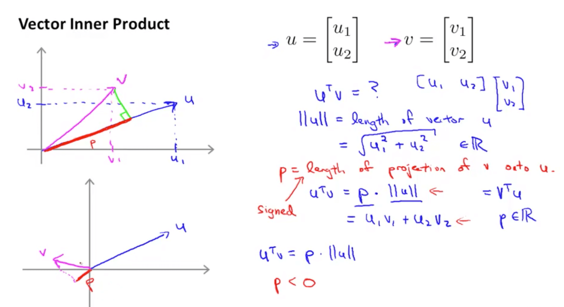
- Vector inner product
- Brief details
- u_transpose * v is also called inner product
- length of u = hypotenuse calculated using Pythagoras’ Theorem
- If we project vector v on vector u (green line)
- p = length of vector v onto u
- p can be positive or negative
- p would be negative when angle between v and u more than 90
- p would be positive when angle between v and u is less than 90
- u_transpose * v = p . ll u ll = u1 v1 + u2 v2 = v_transpose * v
- p = length of vector v onto u
- Brief details
- SVM decision boundary: introduction
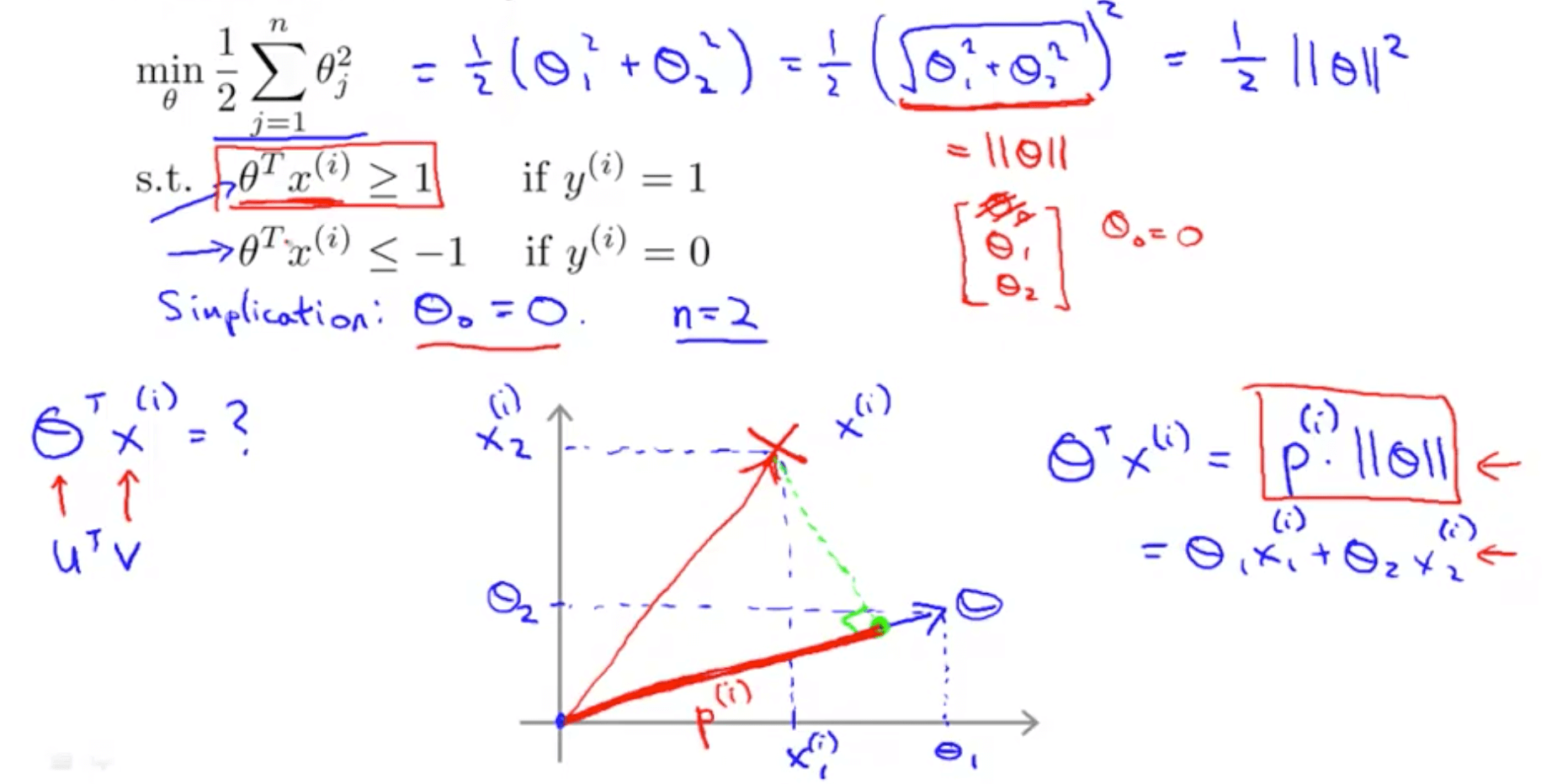
- We set the number of features, n, to 2
- As you can see that normalization in SVM is minimizing the squared norm of the square length of the parameter θ, ll θ ll^2
- SVM decision boundary: projections and hypothesis
- When θ0 = 0, this means the vector passes through the origin
- θ projection will always be 90 degrees to the decision boundary
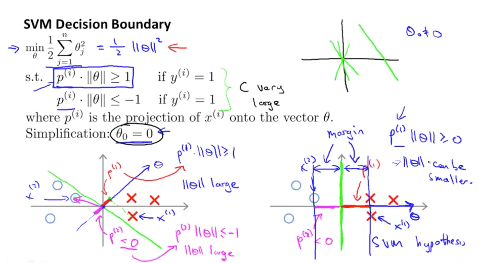
- Decision boundary choice 1: graph on the left
- p1 is projection of x1 example on θ (red)
- p1 . ll θ ll >= 1
- For this to be true ll θ ll has to be large
- p2 is a projection of x2 example on θ (magenta)
- p2 . ll θ ll <= -1
- For this to be true ll θ ll has to be large
- But our purpose is to minimise ll θ ll^2
- This decision boundary choice does not appear to be suitable
- p1 is projection of x1 example on θ (red)
- Decision boundary choice2: graph on the right
- p1 is projection of x1 example on θ (red)
- p1 is much bigger so norm of θ, ll θ ll, can be smaller
- p2 is a projection of x2 example on θ (magenta)
- p2 is much bigger so norm of θ, ll θ ll, can be smaller
- Hence ll θ ll^2 would be smaller
- And this is why SVM would choose this decision boundary
- Magnitude of margin is value of p1, p2, p3 and so on
- SVM would end up with a large margin because it tries to maximize the margin to minimize the squared norm of θ, ll θ ll^2
- p1 is projection of x1 example on θ (red)
2. Kernels
2a. Kernels I
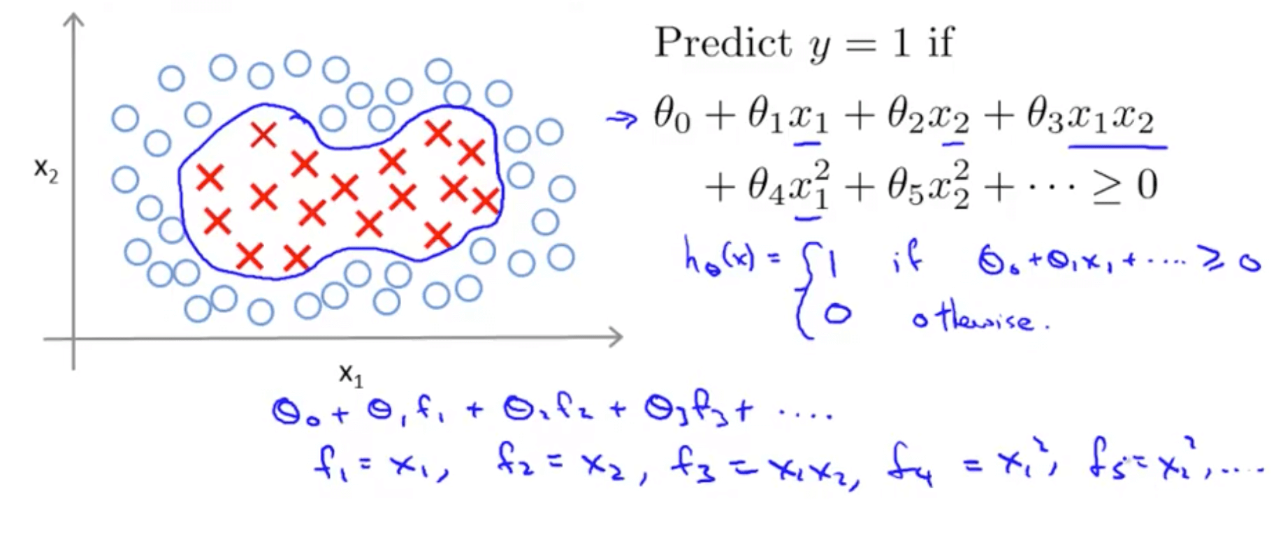
- Non-linear decision boundary
- Given the data, is there a different or better choice of the features f1, f2, f3 … fn?
- We also see that using high order polynomials is computationally expensive
- Gaussian kernel
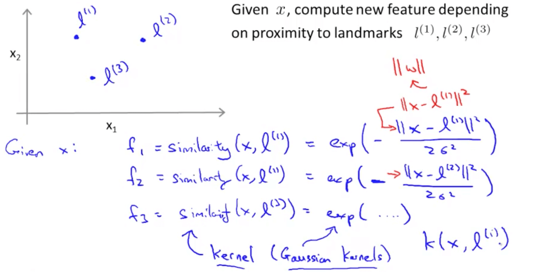
- We will manually pick 3 landmarks (points)
- Given an example x, we will define the features as a measure of similarity between x and the landmarks
- f1 = similarity(x, l(1))
- f2 = similarity(x, l(2))
- f3 = similarity(x, l(3))
- The different similarity functions are Gaussian Kernels
- This kernel is often denoted as k(x, l(i))
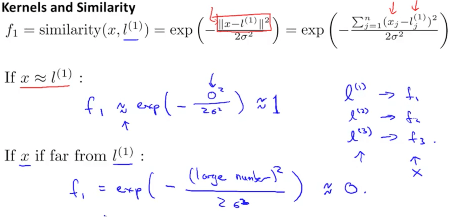
- Kernels and similarity
- Kernel Example
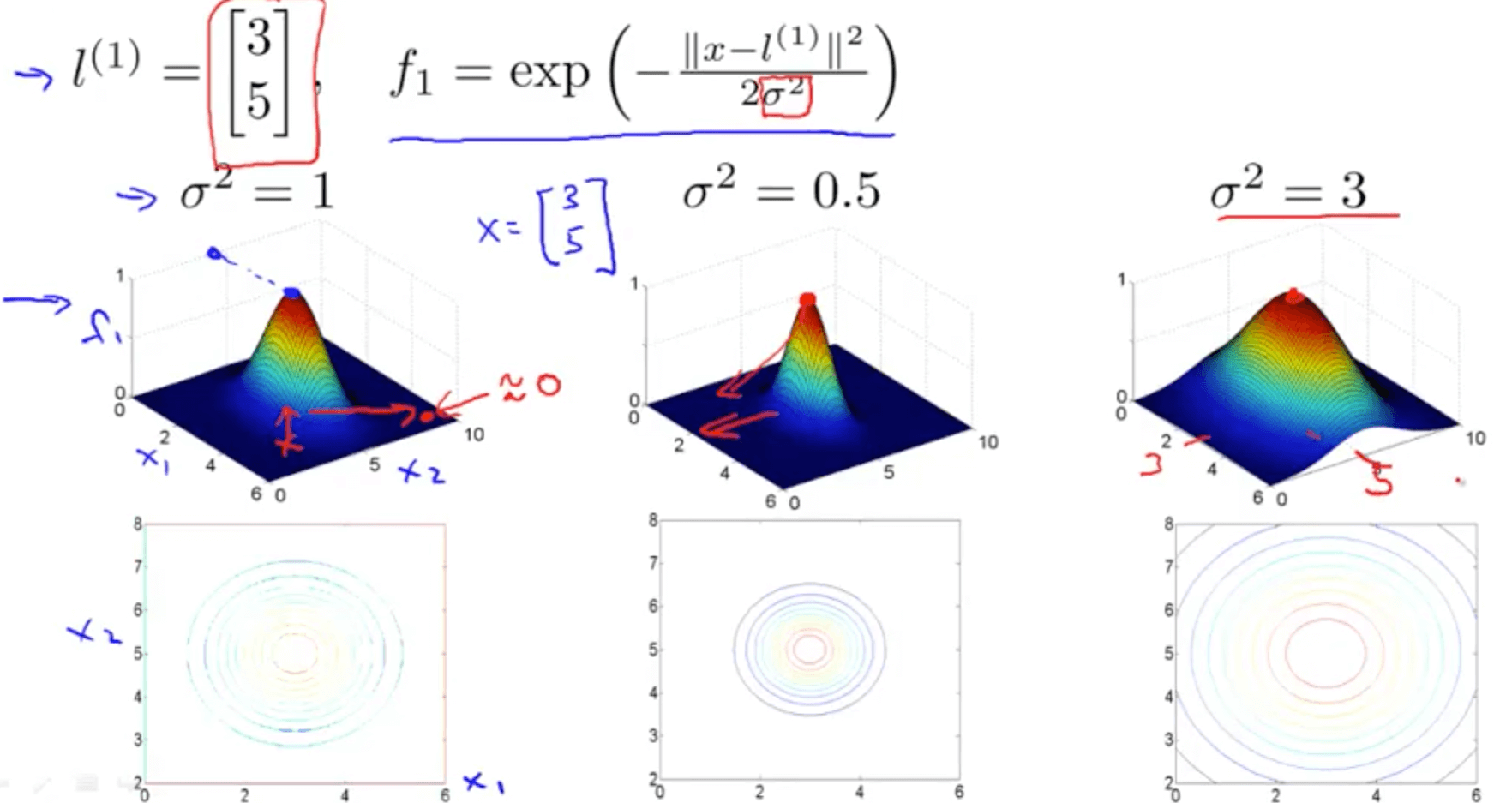
- As you increase sigma square
- As you move away from l1, the value of the feature falls away much more slowly
- As you increase sigma square
- Kernel Example 2
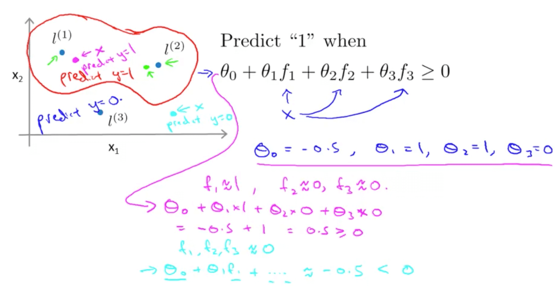
- For the first point (magenta), you will predict 1 because hθ >= 0
- For the second point (cyan), you will predict 0 because hθ < 0
- We can learn complex non-linear decision boundaries
- We predict positive when we’re close to the landmarks
- We predict negative when we’re far away from the landmarks
- Questions we have yet to answer
- How do we get these landmarks?
- How do we choose these landmarks?
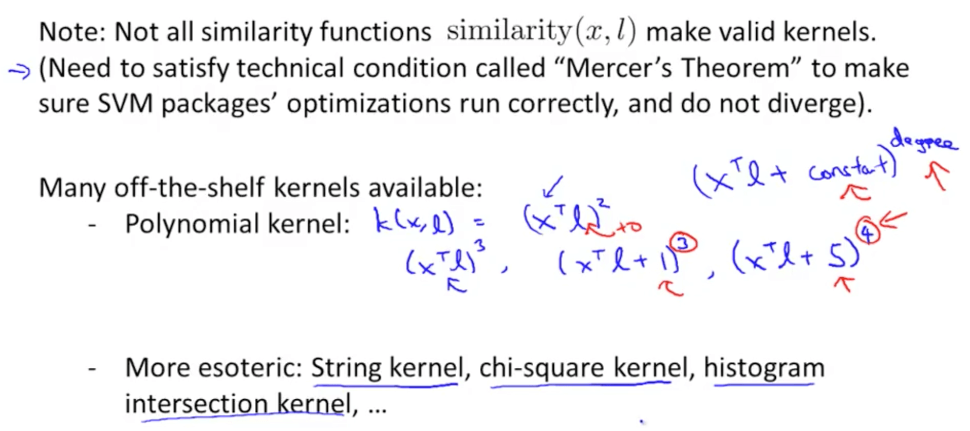
- What other similarity functions can we use beside the Gaussian kernel?
2b. Kernels II
- Choosing the landmarks
- For every training example, we’ll choose the landmarks with the exact locations
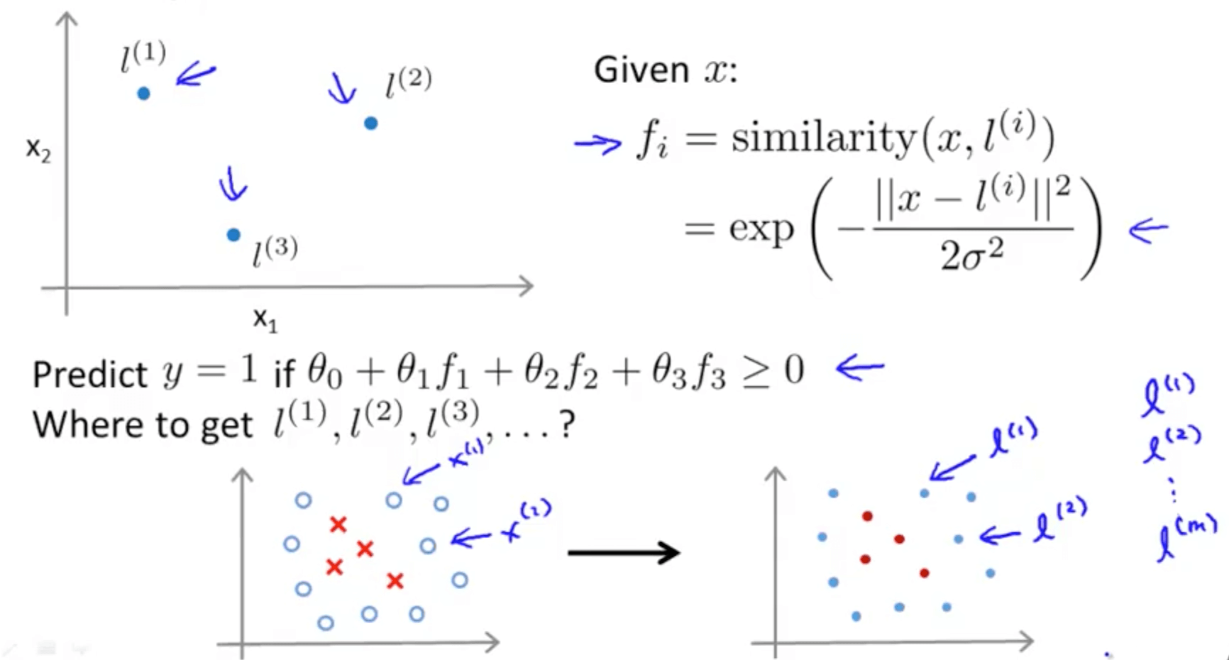
- For every training example, we’ll choose the landmarks with the exact locations
- SVM with kernels
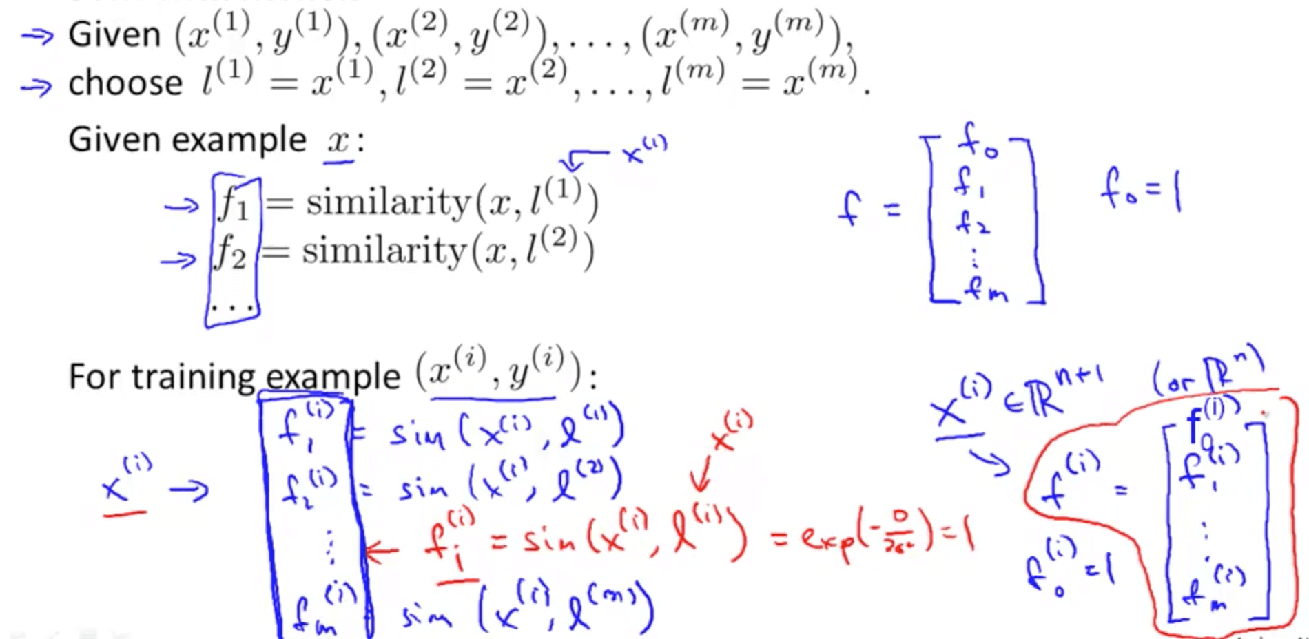
- When we solve the following optimization problem, we get the features
- We do not regularize thetaθ, so it starts from 1
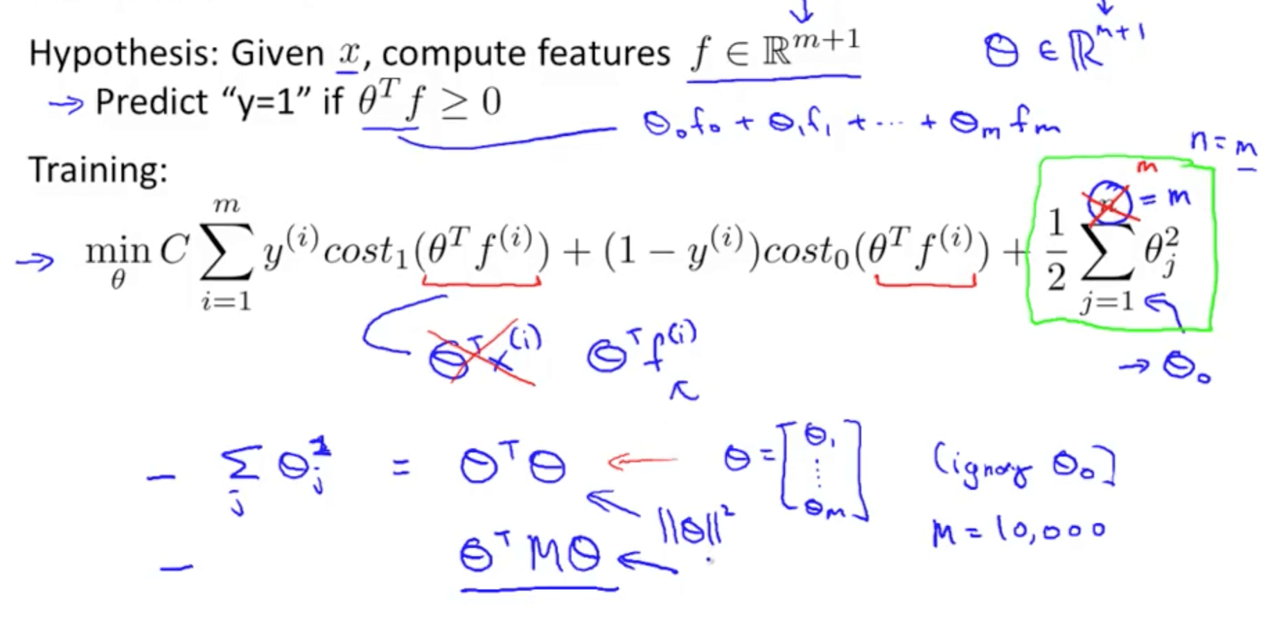
- We do not regularize thetaθ, so it starts from 1
- SVM parameters
3. SVMs in Practice
- We would normally use an SVM software package (liblinear, libsvm etc.) to solve for the parameters θ
- You need to specify the following
- Choice of parameter C
- Choice of kernel (similarity function)
- No kernel is essentially “linear kernel”
- Predict “y = 1” if θ_transpose * x >= 0
- Use this when n is large (number examples) & m is small
- Gaussian kernel
- For this kernel, we have to choose σ^2
- Use this when n is small (number of examples) and/or m is large
- No kernel is essentially “linear kernel”
- If you choose a Gaussian kernel
- Octave implementation
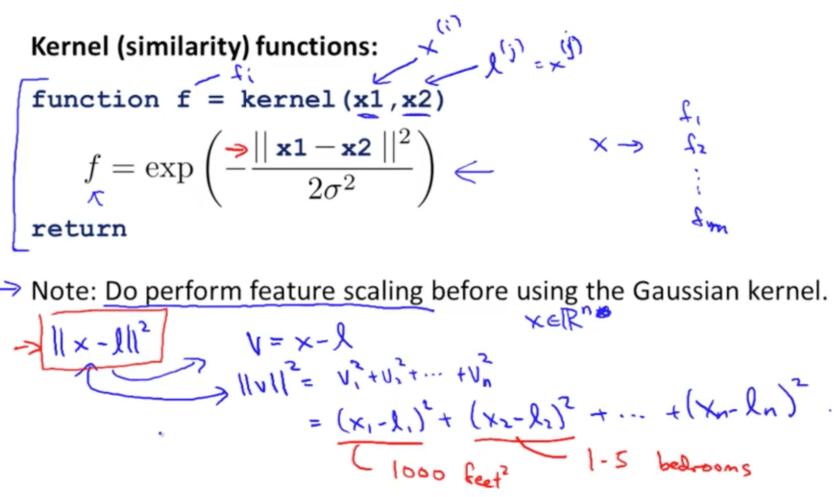
- We have to do feature scaling before using Gaussian kernel
- This is because if we don’t, ll x - l ll^2 would be dominated mainly by the features that are large in scale such as the 1000sqft feature
- The Gaussian kernel is also parameterized by a bandwidth pa- rameter, σ, which determines how fast the similarity metric decreases (to 0) as the examples are further apart
- We have to do feature scaling before using Gaussian kernel
- Octave implementation
- Other choices of kernel
- Multi-class classification
- Typically most packages have this function
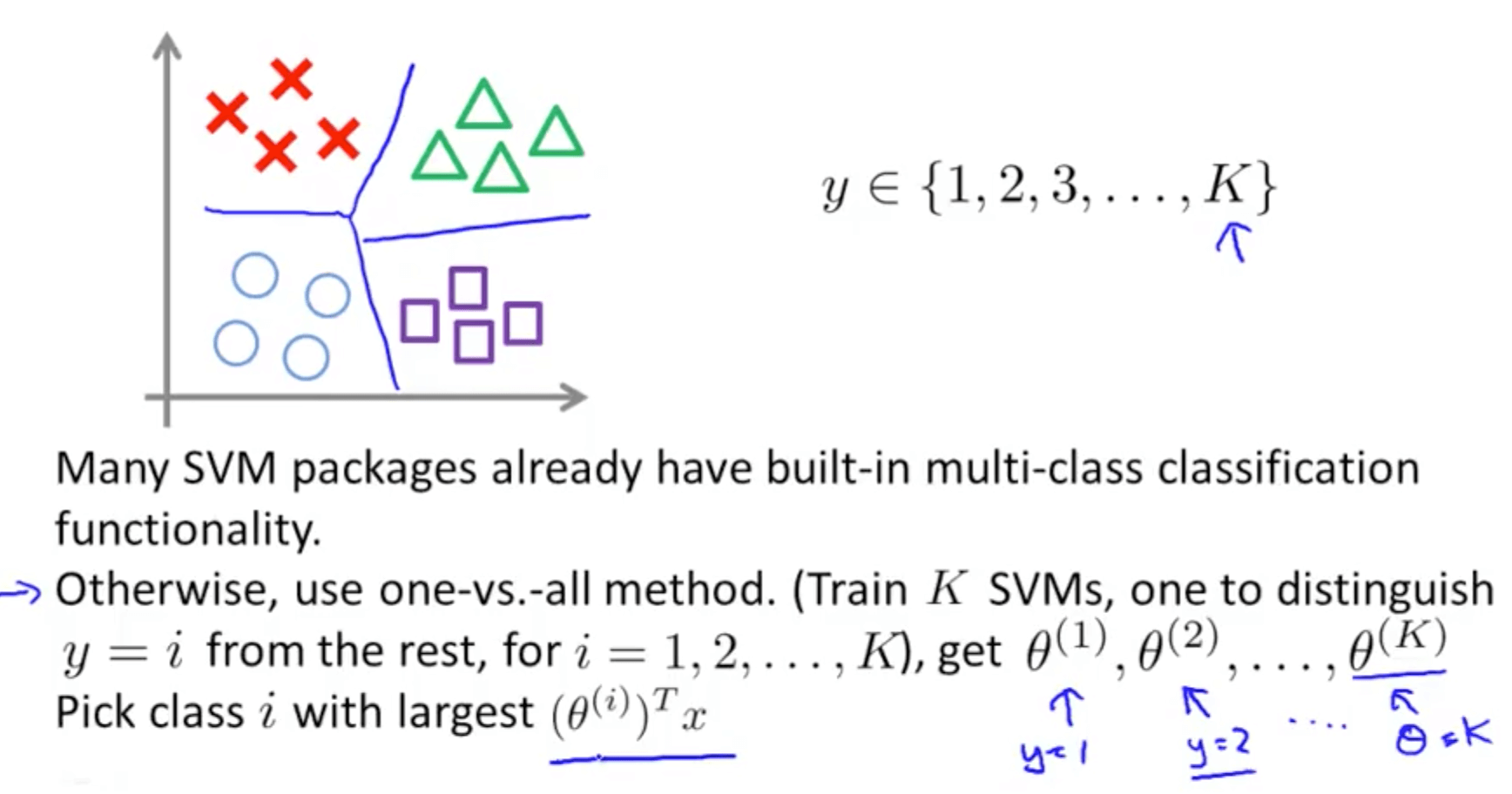
- Typically most packages have this function
- Logistic Regression vs SVMs
- When do we use logistic regression and when do we use SVMs?
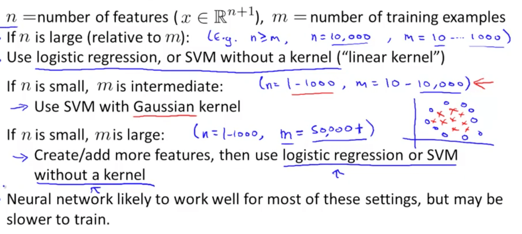
- The key thing to note is that if there is a huge number of training examples, a Gaussian kernel takes a long time
- The optimization problem of an SVM is a convex problem, so you will always find the global minimum
- Neural Network: non-convex, may find local optima
- When do we use logistic regression and when do we use SVMs?