Non-linear hypothesis, neurons and the brain, model representation, and multi-class classification.
1. Motivations
I would like to give full credits to the respective authors as these are my personal python notebooks taken from deep learning courses from Andrew Ng, Data School and Udemy :) This is a simple python notebook hosted generously through Github Pages that is on my main personal notes repository on https://github.com/ritchieng/ritchieng.github.io. They are meant for my personal review but I have open-source my repository of personal notes as a lot of people found it useful.
1a. Non-linear Hypothesis
- You can add more features
- But it will be slow to process
- If you have an image with 50 x 50 pixels (greyscale, not RGB)
- n = 50 x 50 = 2500
- quadratic features = (2500 x 2500) / 2
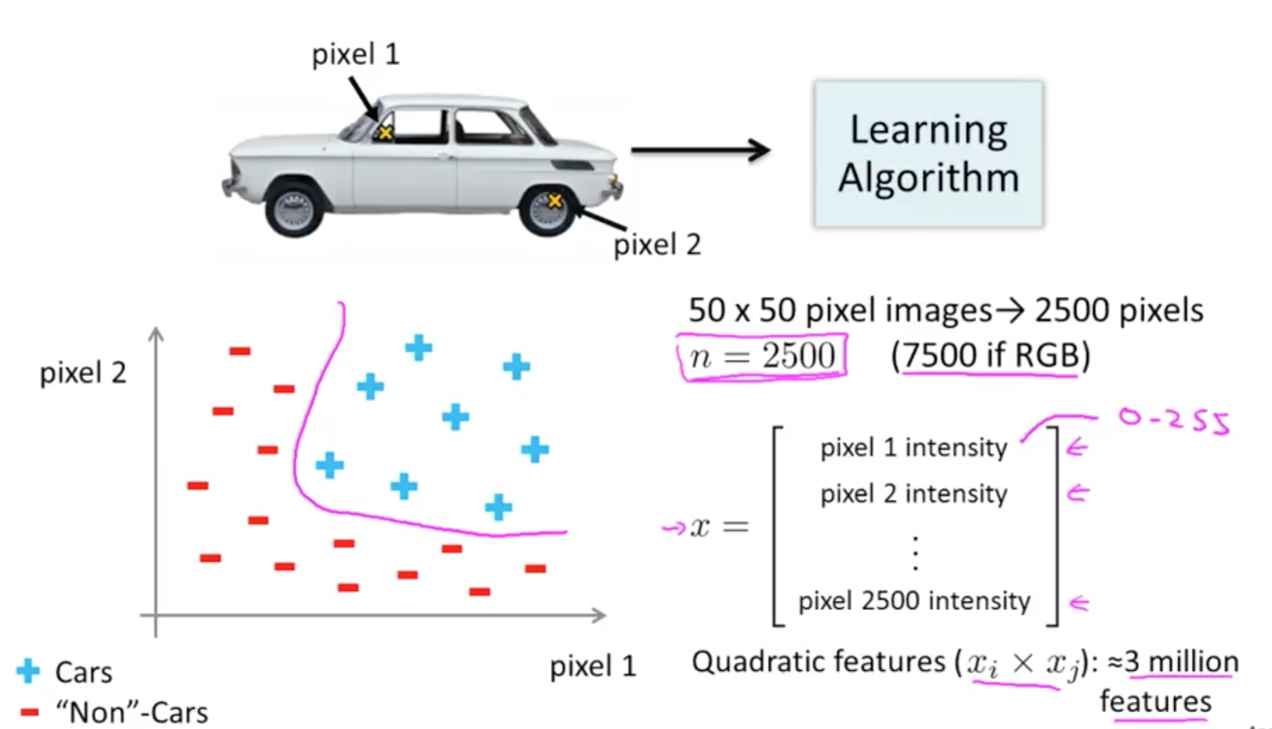
- Neural networks are much better for a complex nonlinear hypothesis
1b. Neurons and the Brain
- Origins
- Algorithms that try to mimic the brain
- Was very widely used in the 80s and early 90’s
- Popularity diminished in the late 90’s
- Recent resurgence
- State-of-the-art techniques for many applications
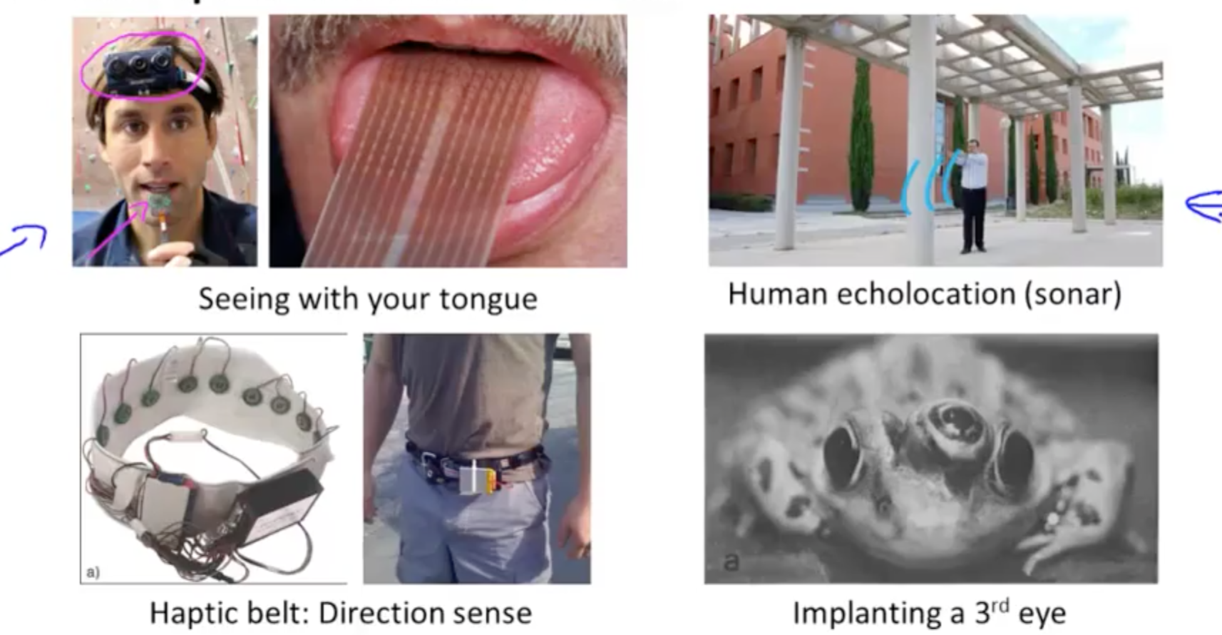
- The “one learning algorithm” hypothesis
- Auditory cortex handles hearing
- Re-wire to learn to see
- Somatosensory cortex handles feeling
- Re-wire to learn to see
- Plug in data and the brain will learn accordingly
- Auditory cortex handles hearing
- Examples of learning
2. Neural Networks
2a. Model Representation I
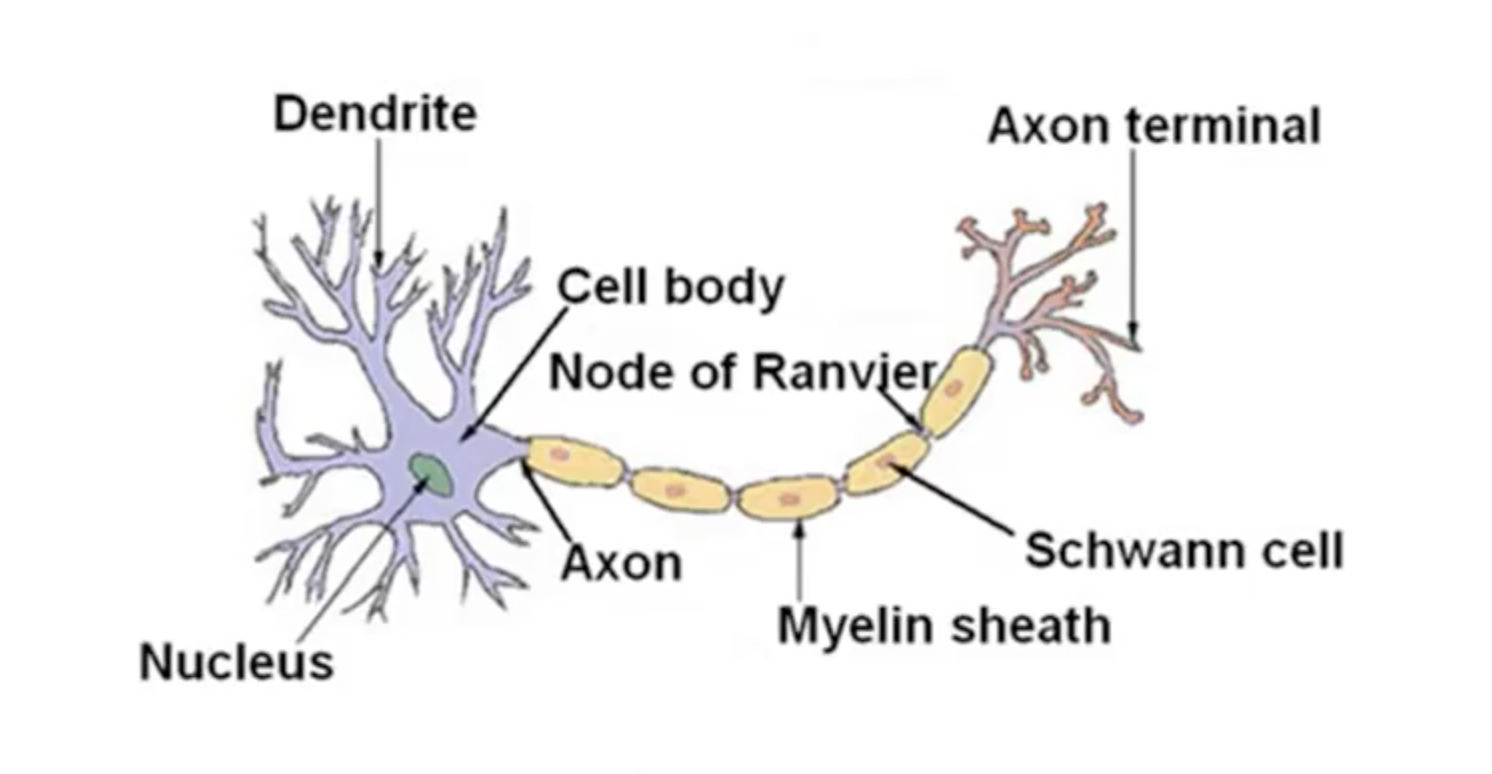
- Neuron in the brain
- Many neurons in our brain
- Dendrite: receive input
- Axon: produce output
- When it sends a message through the Axon to another neuron
- It sends to another neuron’s Dendrite
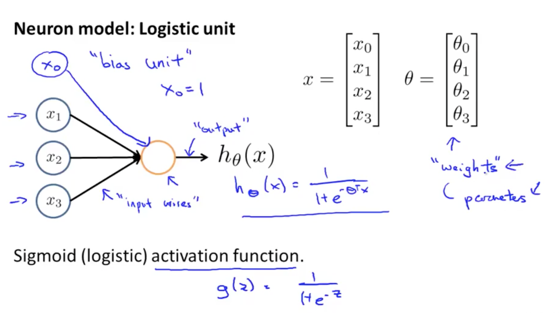
- Neuron model: logistic unit
- Yellow circle: body of neuron
- Input wires: dendrites
- Output wire: axon
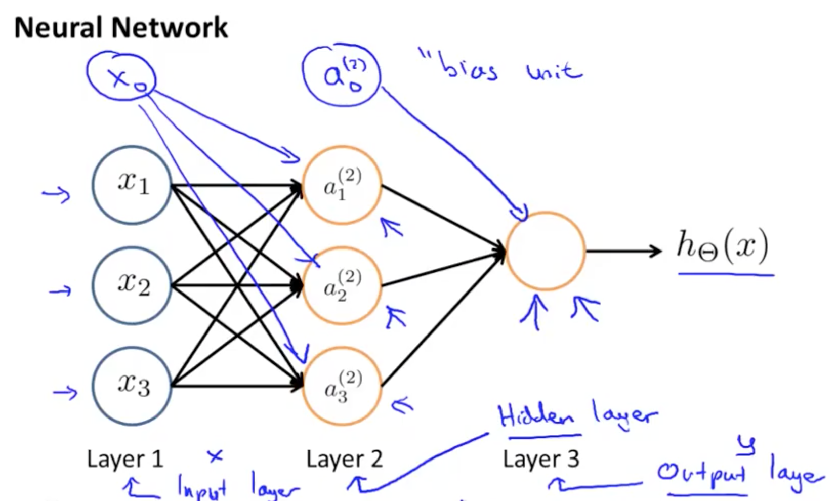
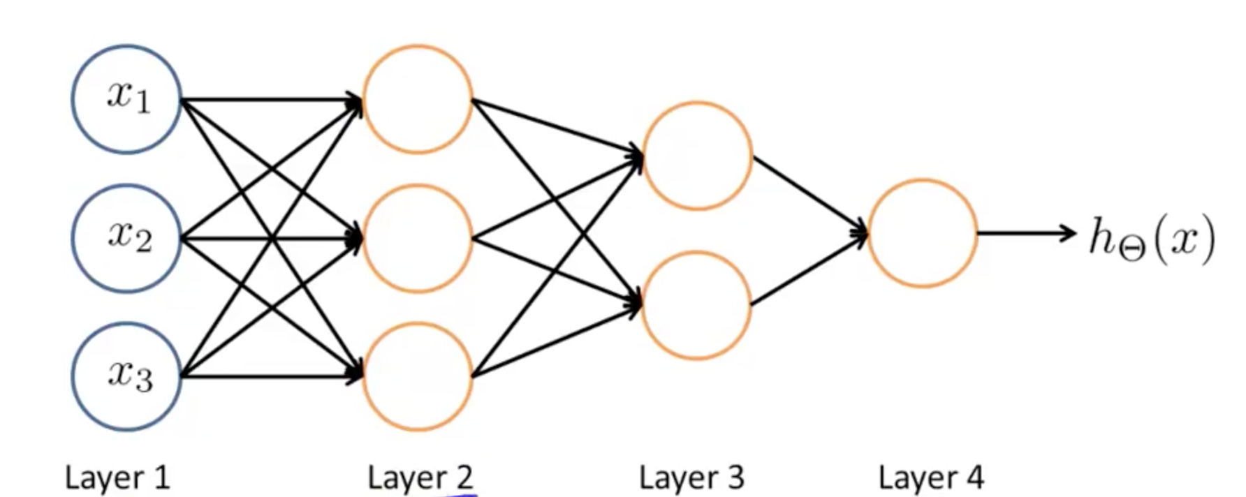
- Neural Network
- 3 Layers
- 1 Layer: input layer
- 2 Layer: hidden layer
- Unable to observe values
- Anything other than input or output layer
- 3 Layer: output layer
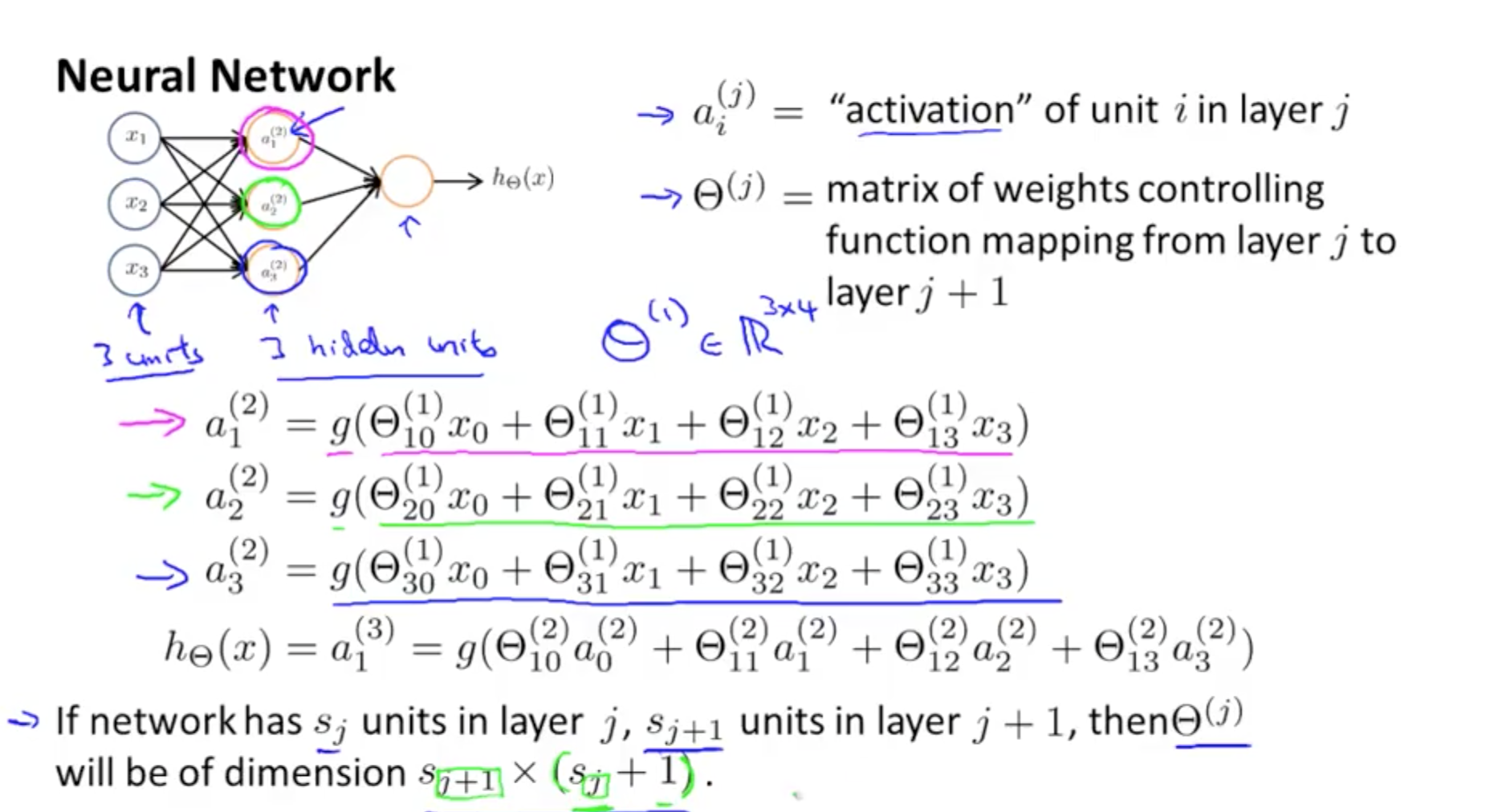
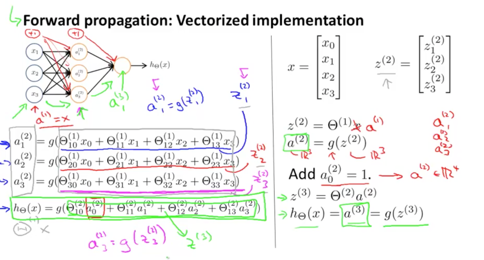
- We calculate each of the layer-2 activations based on the input values with the bias term (which is equal to 1)
- i.e. x0 to x3
- We then calculate the final hypothesis (i.e. the single node in layer 3) using exactly the same logic, except in input is not x values, but the activation values from the preceding layer
- The activation value on each hidden unit (e.g. a12 ) is equal to the sigmoid function applied to the linear combination of inputs
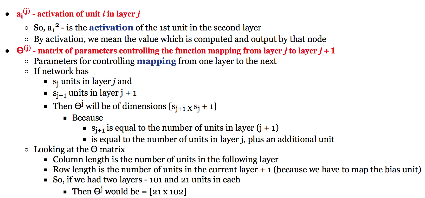
- Three input units
- Ɵ(1) is the matrix of parameters governing the mapping of the input units to hidden units
- Ɵ(1) here is a [3 x 4] dimensional matrix
- Three hidden units
- Then Ɵ(2) is the matrix of parameters governing the mapping of the hidden layer to the output layer
- Ɵ(2) here is a [1 x 4] dimensional matrix (i.e. a row vector)
- Then Ɵ(2) is the matrix of parameters governing the mapping of the hidden layer to the output layer
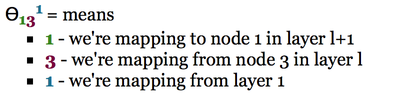
- Every input/activation goes to every node in following layer
- Which means each “layer transition” uses a matrix of parameters with the following significance

- j (first of two subscript numbers)= ranges from 1 to the number of units in layer l+1
- i (second of two subscript numbers) = ranges from 0 to the number of units in layer l
- l is the layer you’re moving FROM
- Which means each “layer transition” uses a matrix of parameters with the following significance
- 3 Layers
- Notation
2a. Model Representation II
- Here we’ll look at how to carry out the computation efficiently through a vectorized implementation. We’ll also consider why neural networks are good and how we can use them to learn complex non-linear things
- Forward propagation: vectorized implementation
- g applies sigmoid-function element-wise to z
- This process of calculating H(x) is called forward propagation
- Worked out from the first layer
- Starts off with activations of input unit
- Propagate forward and calculate the activation of each layer sequentially
- Similar to logistic regression if you leave out the first layer
- Only second and third layer
- Third layer resembles a logistic regression node
- The features in layer 2 are calculated/learned, not original features
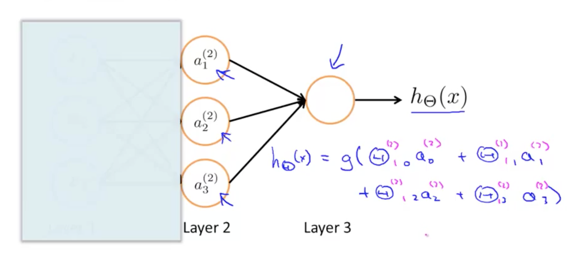
- Neural network, learns its own features
- The features a’s are learned from x’s
- It learns its own features to feed into logistic regression
- Better hypothesis than if we were constrained with just x1, x2, x3
- We can have whatever features we want to feed to the final logistic regression function
- Implemention in Octave for a2
a2 = sigmoid (Theta1 * x);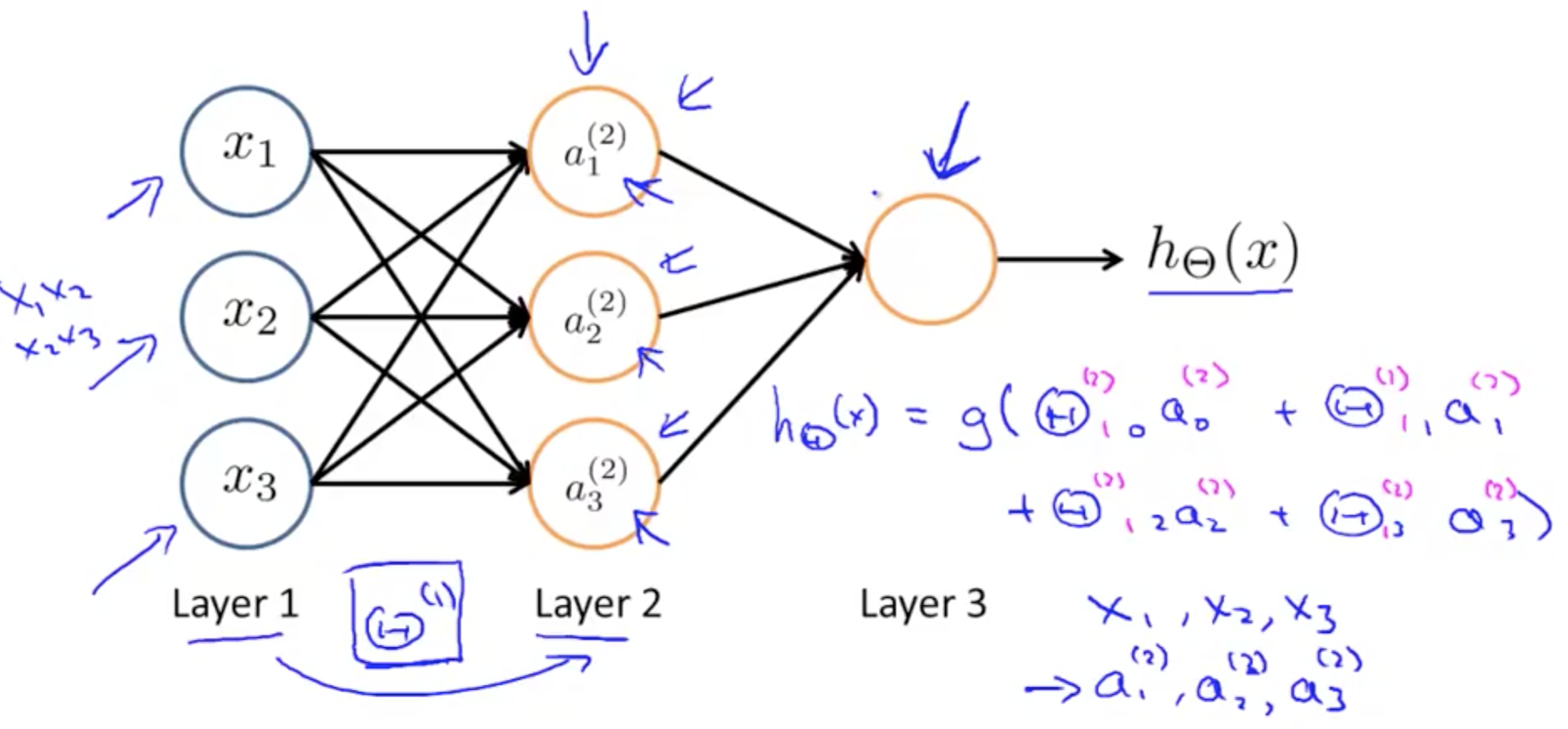
- Other network architectures
- Layer 2 and 3 are hidden layers
- Layer 2 and 3 are hidden layers
2. Neural Network Application
2a. Examples and Intuitions I
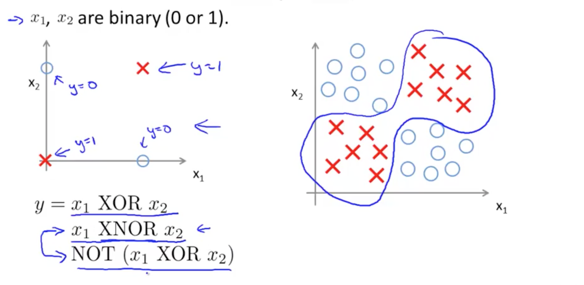
- XOR/XNOR
- XOR: or
- XNOR: not or
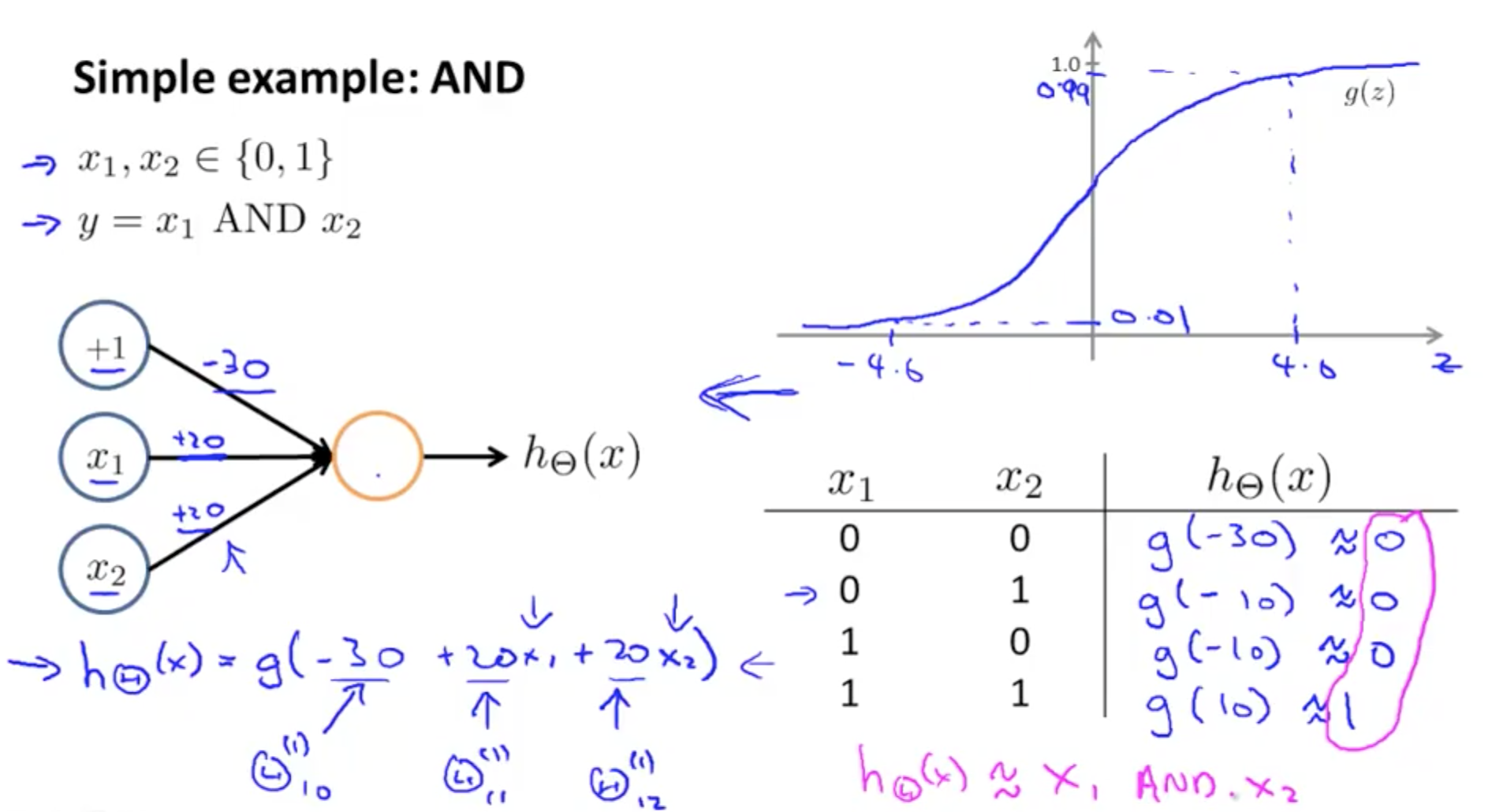
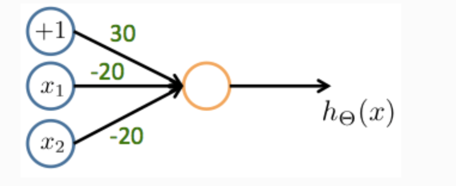
- AND function
- Outputs 1 only if x1 and x2 are 1
- Draw a table to determine if OR or AND
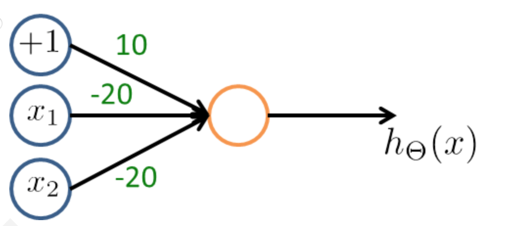
- NAND function
- NOT AND
- NOT AND
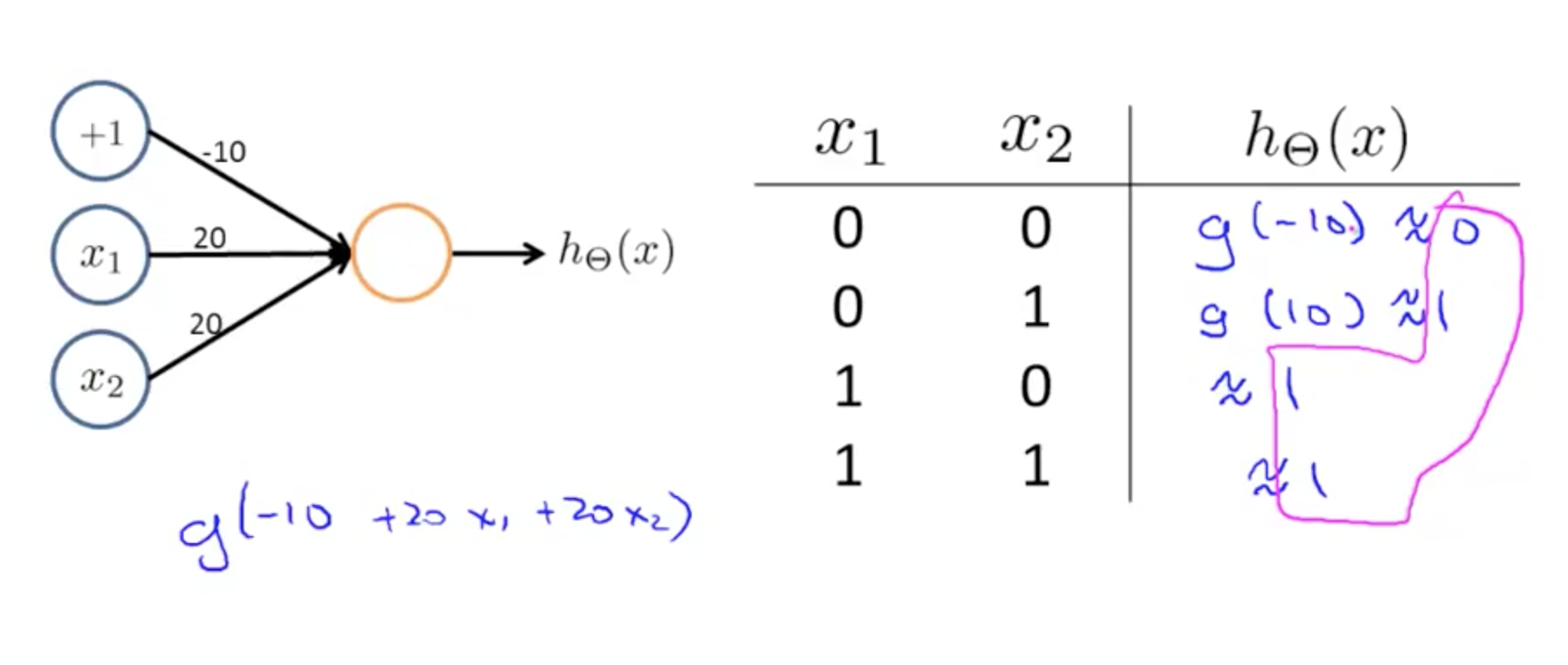
- OR function
2b. Examples and Intuitions II
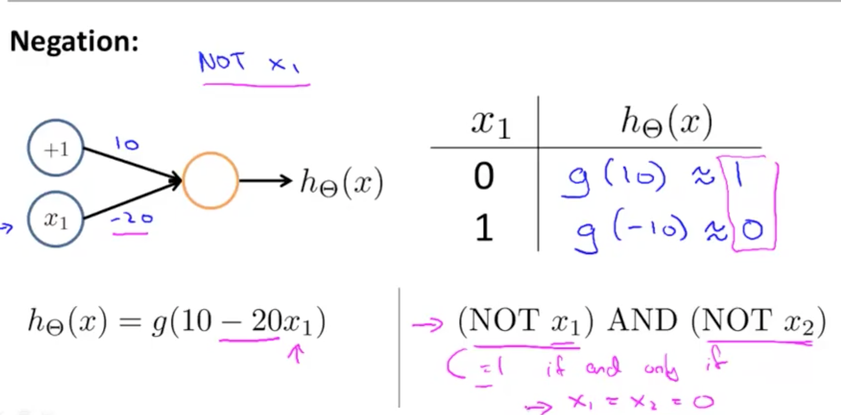
- NOT function
- XNOR function
- NOT XOR
- NOT an exclusive or
- Hence we would want
- AND
- Neither
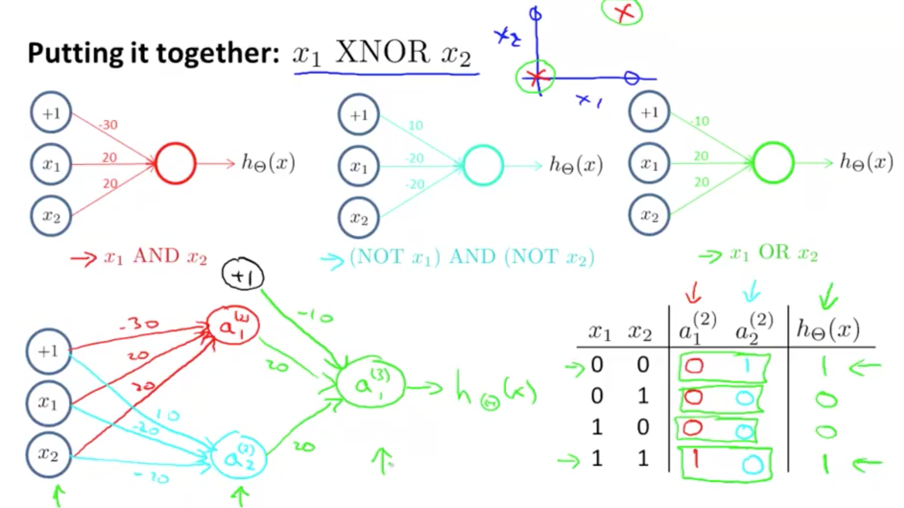
- Hence we would want
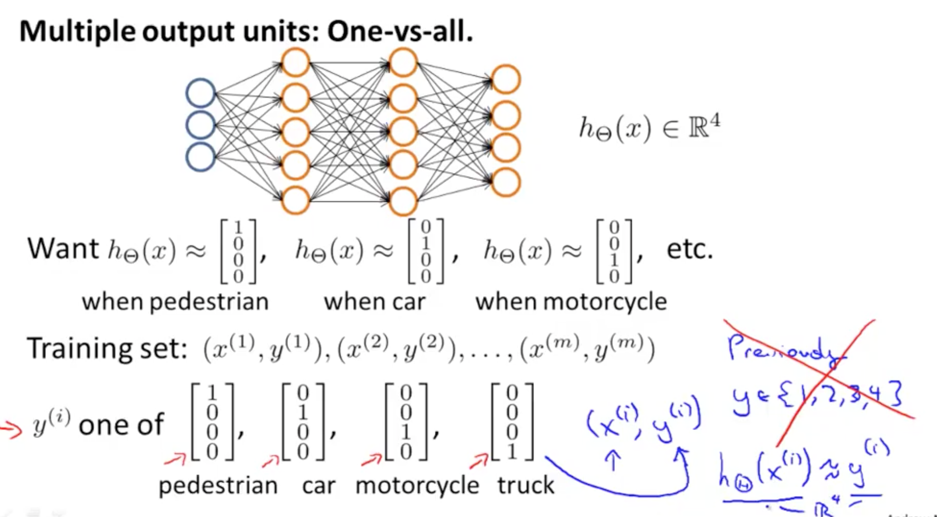
2c. Multi-class Classification
- Example: identify 4 classes
- You would want a 4 x 1 vector for h_theta(X)
- 4 logistic regression classifiers in the output layer
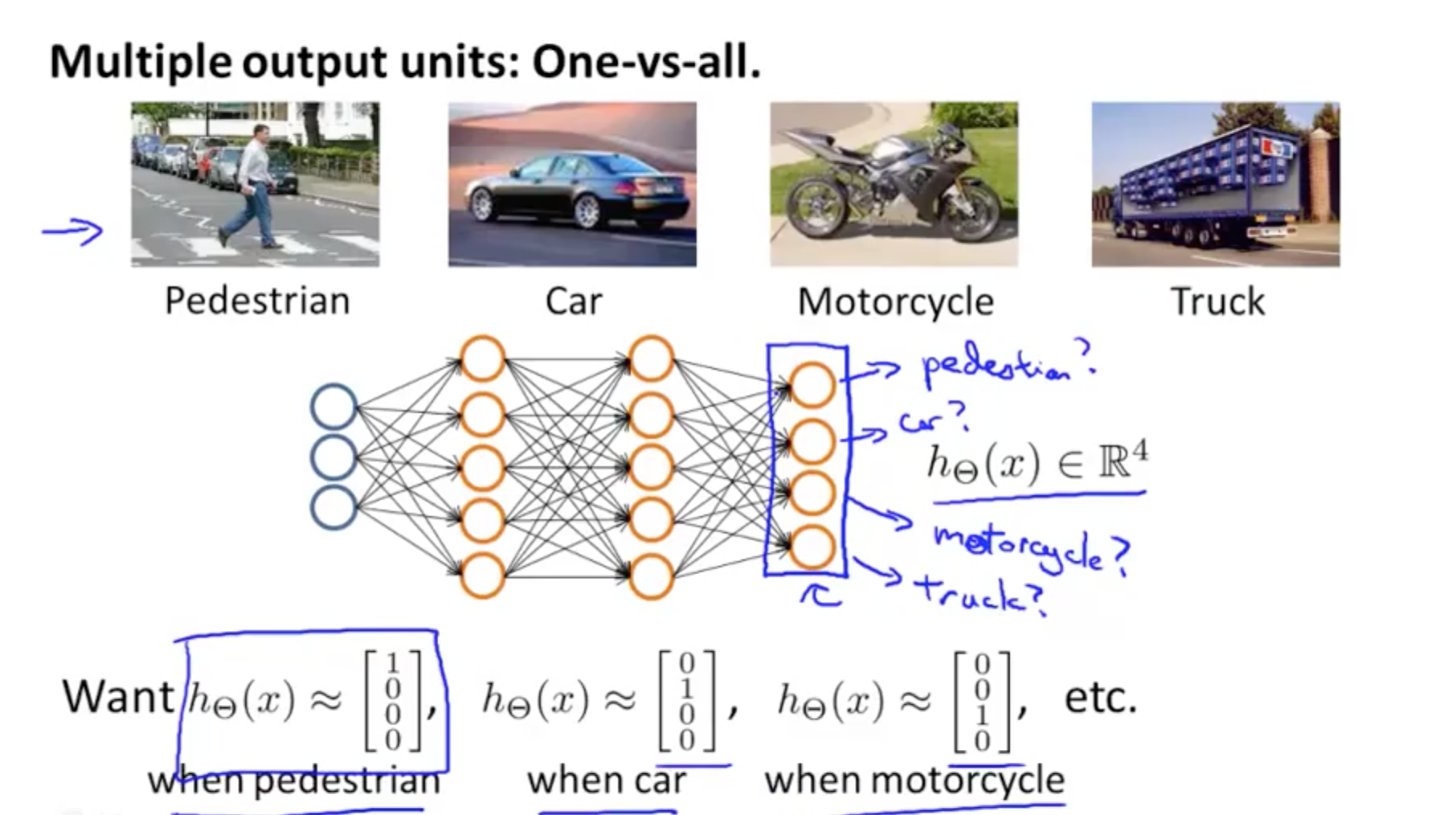
- There will be 4 output
- y would be a 4 x 1 vector instead of an integer