Similarities to normal neural networks and supervised learning.
Deep Learning: Introduction
Pedestrian Detection Example
- We can use a binary classifier of pedestrian and no pedestrian.
- Then we slide a "window" across all possible locations in the image to detect if there is a pedestrian.
Web Search Ranking Example
- Take pair of query and webpage.
- We then classify as relevant or not relevant.
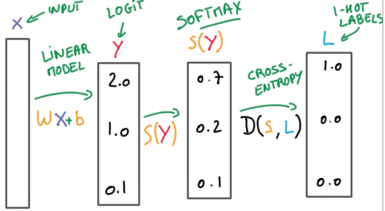
Logistic Classifier (Linear Classifier)
- $$ Wx + b = y $$
- We take inputs as a vector x, and multiply it by the weights matrix W, the we add the bias vector b to produce y, output which is a matrix/vector of scores.
Softmax function
- We can turn scores (logits) into probabilities using a softmax function.
- The probabilities will all sum to 1.
- Probability will be low if it's a high score.
- Probability will be high if it's a low score.
- $$ S(y_i) = \frac {e^{y_i}} {\sum_j e^{y_j}} $$
In [2]:
"""Softmax Function"""
# Your softmax(x) function should
# return a NumPy array of the same shape as x.

scores = [3.0, 1.0, 0.2]

import numpy as np

def softmax(x):
    """Compute softmax values for each sets of scores in x."""
    # TODO: Compute and return softmax(x)
    # We sum across the row.
    soft_max = np.exp(x) / np.sum(np.exp(x), axis=0)
    return soft_max


# Probabilities should sum to 1.
print(softmax(scores))

# Plot softmax curves
import matplotlib.pyplot as plt
x = np.arange(-2.0, 6.0, 0.1)
scores = np.vstack([x, np.ones_like(x), 0.2 * np.ones_like(x)])

plt.plot(x, softmax(scores).T, linewidth=2)
plt.show()

In [3]:
# Multiply scores by 10.
scores = np.array([3.0, 1.0, 0.2])
print(softmax(scores * 10))
Probabilities get close to either 1.0 or 0.0.
In [5]:
# Divide scores by 10.
scores = np.array([3.0, 1.0, 0.2])
print(softmax(scores / 10))
- Probabilities get cose to the uniform distribution because since all the scores decrease in magnitude, the resulting softmax probabilities will be closer to each other.
- We want to be confident over time from this to the above with more data.

One-Hot Encoding
- We want the output to be 1 or 0. This is basically one-hot encoding.
Cross-Entropy
- $$ D(S, L) = - \sum_i L_i log(S_i) $$
- It is a loss function.
- In some rough sense, the cross-entropy is measuring how inefficient our predictions are for describing the truth.
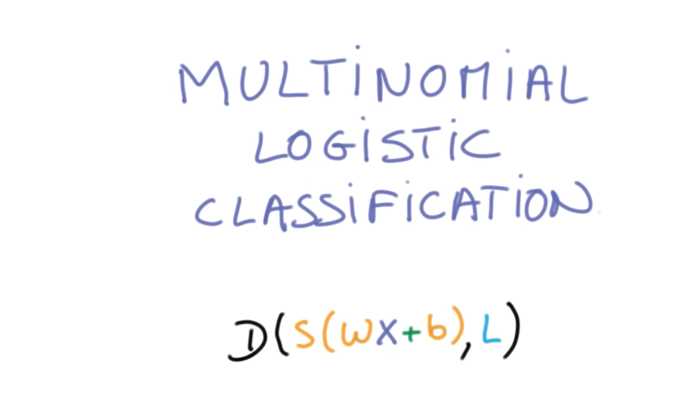
Putting everything together, we get the following which is essentially multinomial logistic regression or softmax logistic regression.
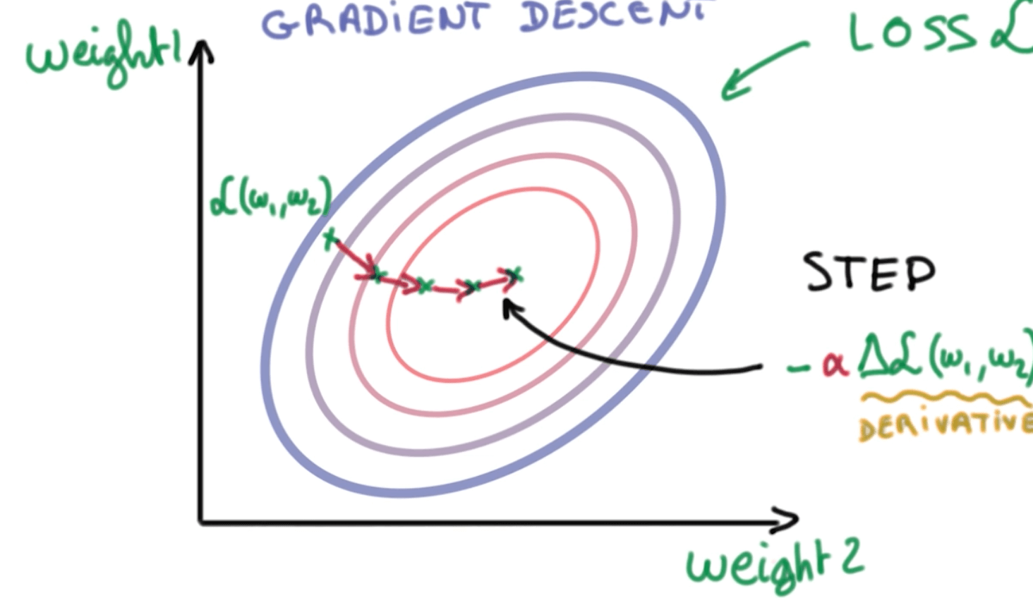
Training loss
- How do we find weights w and bias b to have low distance for correct class and high distance for incorrect class.
- We can do this using a training loss function.
- We want to minimize the following loss function.
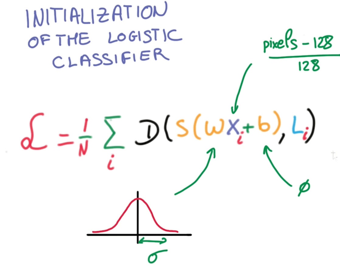
- $$ L = \frac {1}{n} \sum_i D(S(wx_i + b), \ L_i) $$
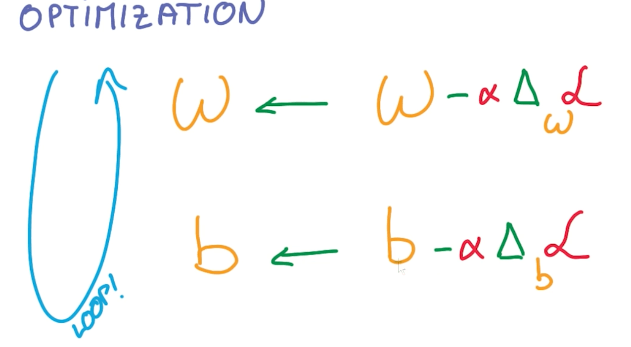
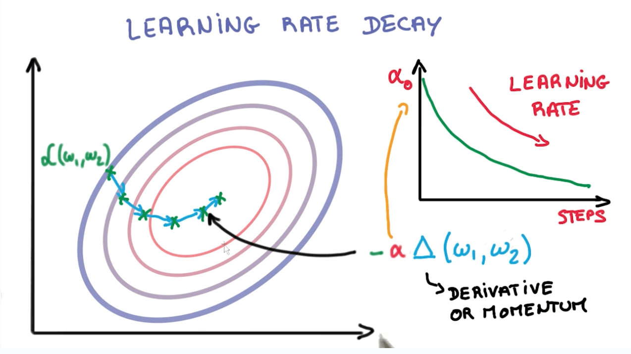
- Minimize loss graph based on two weights by taking small steps called gradient descent.
- We take the derivative of the loss with respect to our parameters.
Numerical Stability
- Adding very small values to a large value would introduce problems.
- We would always want the following:
- Well conditioned
- Mean: $ X_i = 0 $
- Variance: $\sigma(X_i) = \sigma(X_j)$
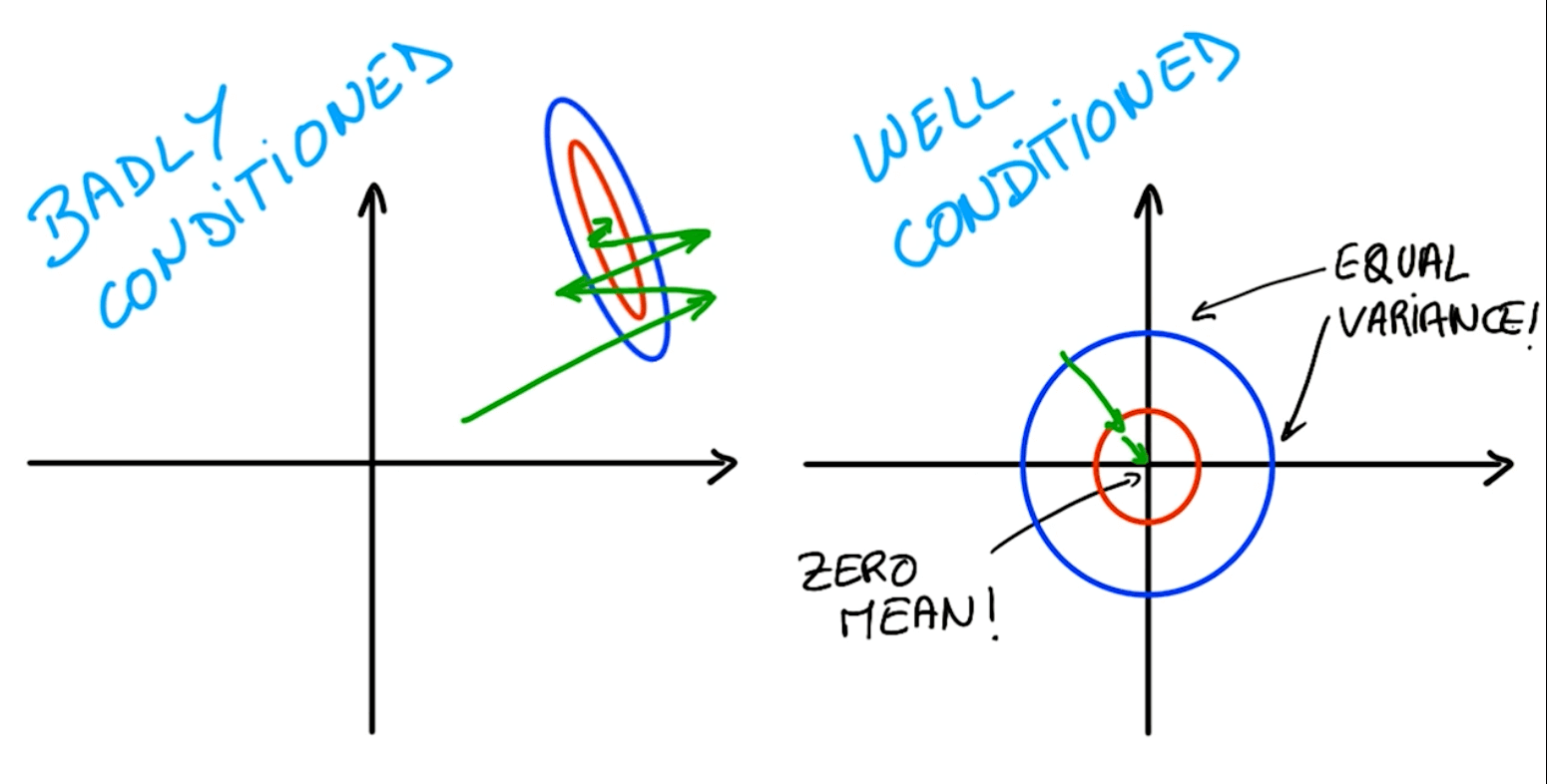
- Optimizer don't have to do a lot of searching
- We can do this with image.
- Take pixel value (0 to 255)
- Subtract 128 and divide by 128.
- We can do this with image.
- Random weight initialization
- Draw weights randomly with a Gaussian distribution and standard deviation $\sigma$
- We can start with small $\sigma$ (uncertain)
- Draw weights randomly with a Gaussian distribution and standard deviation $\sigma$
- Well conditioned
What do we have now?
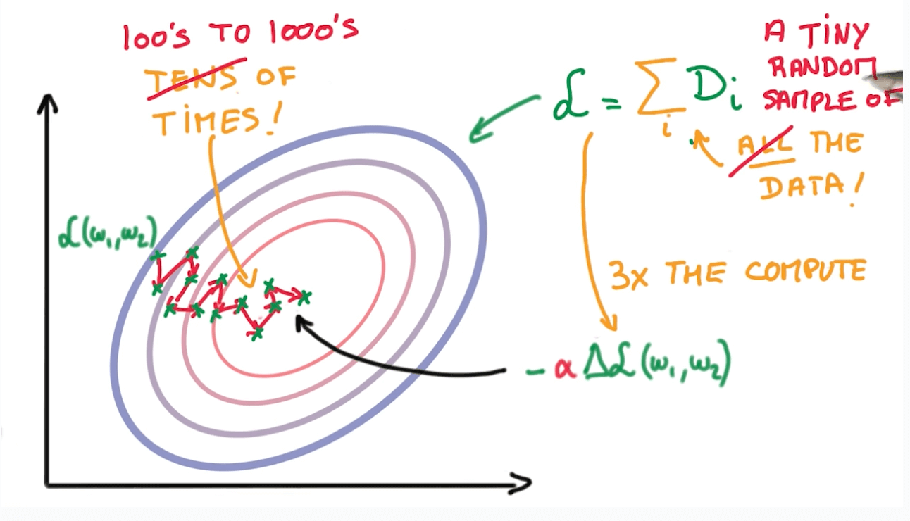
Stochastic Gradient Descent
- If we use samples, it's faster than running Gradient Descent on the whole data.
- We can take many random groups of samples and calculate the averages.
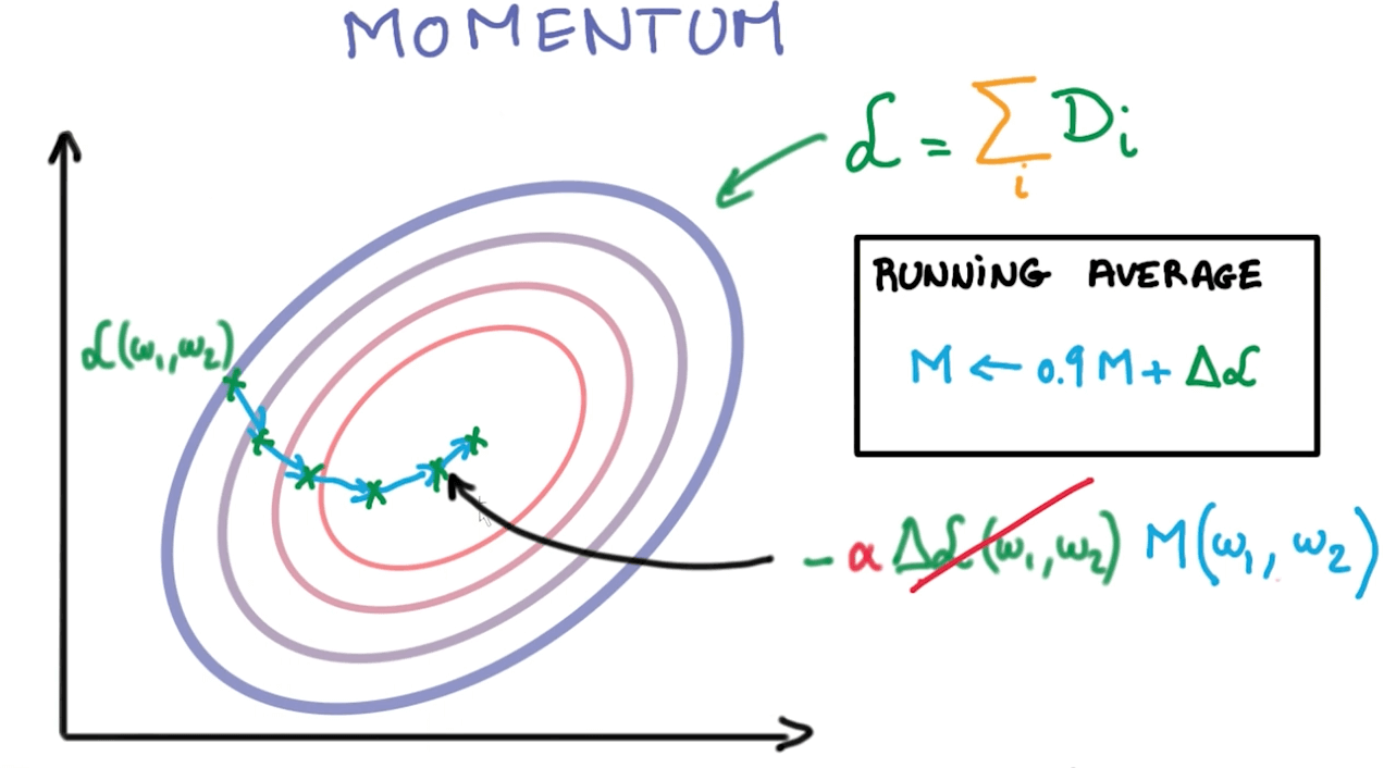
Momentum
- Unlike in classical stochastic gradient descent, it tends to keep traveling in the same direction, preventing oscillations.
- We can reach convergence faster.
Learning rate decay
- It's better to make the step smaller with each step.
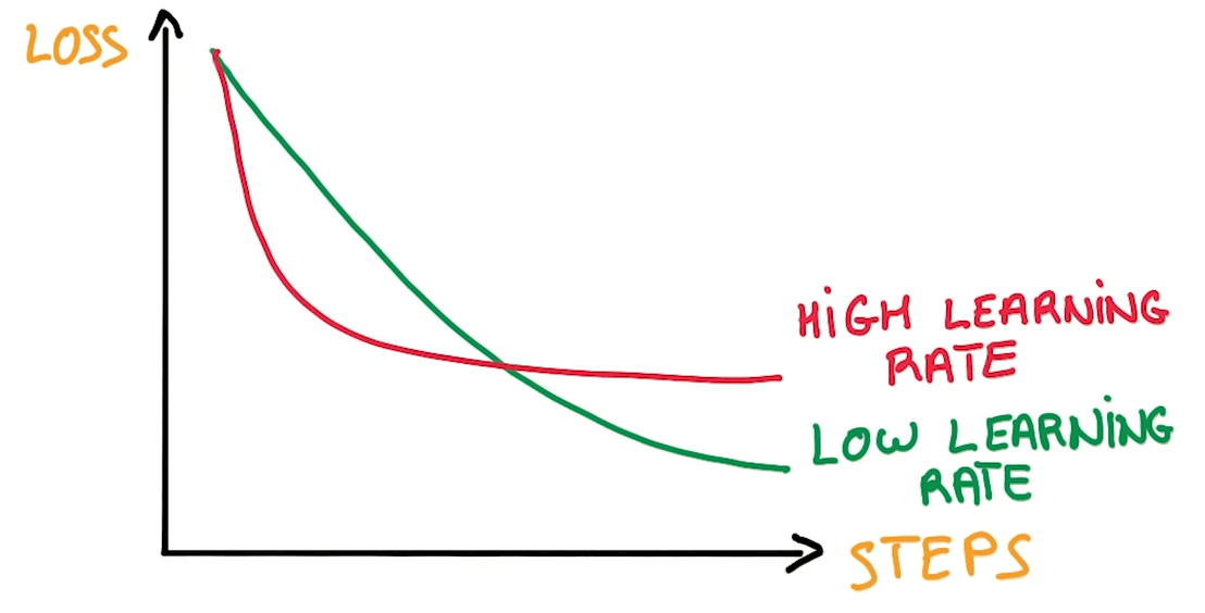
Learning rate tuning
Benefits of SGD
- Many hyperparameters to play with
- Initial learning rate
- If things are wrong, try to lower learning rate
- Learning rate decay
- Momentum
- Batch size
- Weight initialization
- Initial learning rate
Alternative: Adagrad
- It does the following 3 implicitly:
- Initial learning rate
- Learning rate decay
- Momentum.
- It can be a little worst than a precisely tuned SGD.
- But you can use it to move fast.