Gradient descent with large data, stochastic gradient descent, mini-batch gradient descent, map reduce, data parallelism, and online learning.
1. Gradient Descent with Large Data Sets
I would like to give full credits to the respective authors as these are my personal python notebooks taken from deep learning courses from Andrew Ng, Data School and Udemy :) This is a simple python notebook hosted generously through Github Pages that is on my main personal notes repository on https://github.com/ritchieng/ritchieng.github.io. They are meant for my personal review but I have open-source my repository of personal notes as a lot of people found it useful.
1a. Learning with Large Data Sets
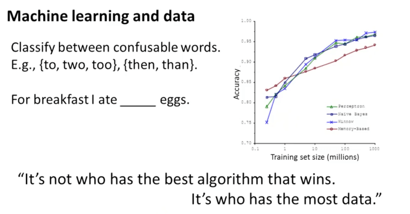
- Why do we want large data set?
- This is evident when we take a low-bias learning algorithm and train it on a lot of data
- The example of how “I ate two (two) eggs” shows how the algorithm performs well when we feed it a lot of data
- The example of how “I ate two (two) eggs” shows how the algorithm performs well when we feed it a lot of data
- This is evident when we take a low-bias learning algorithm and train it on a lot of data
- Learning with large data sets has computational problems
- If m = 100m, we have to sum over 100m entries to compute one step of gradient descent
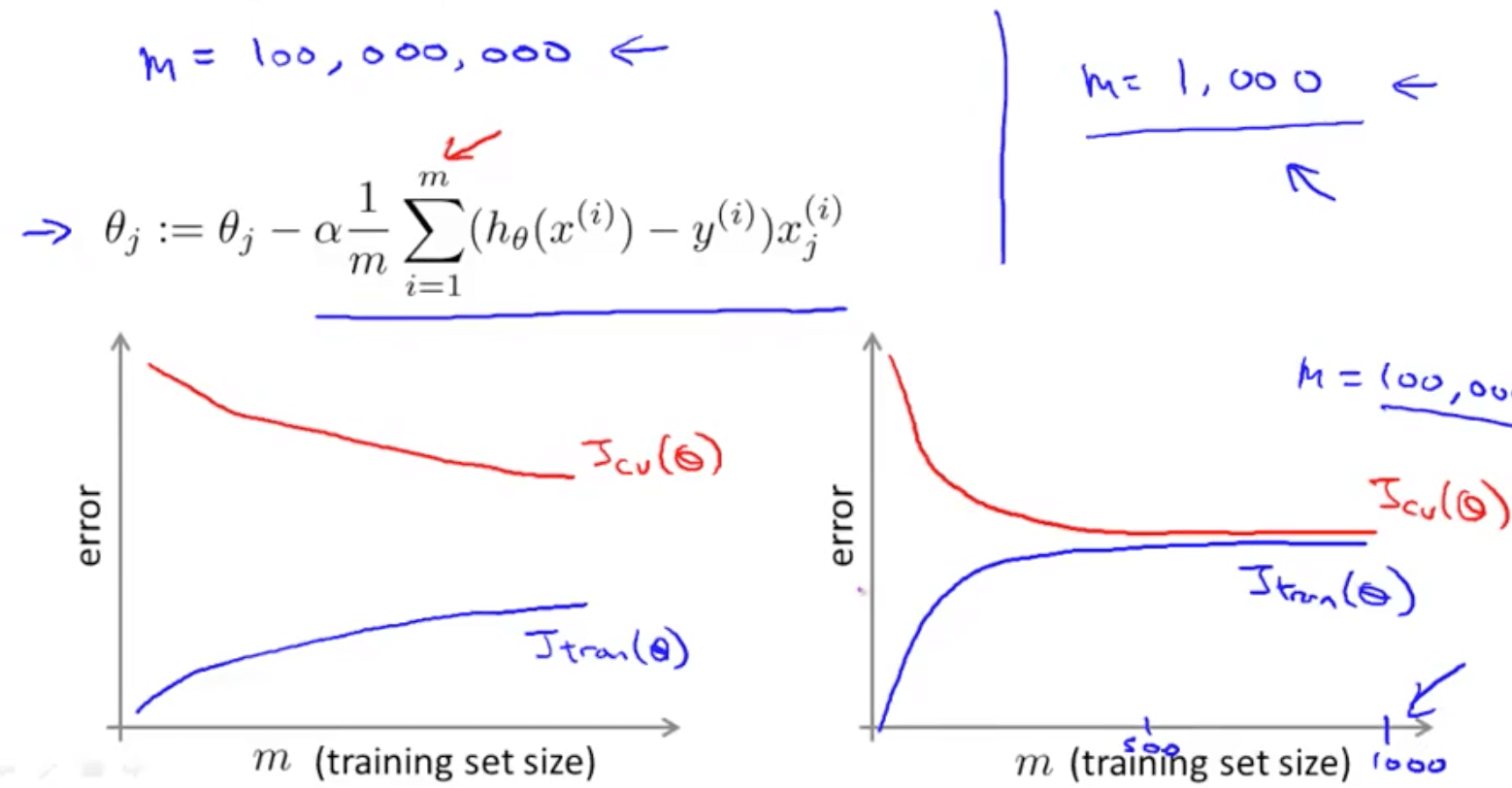
- Suppose you are facing a supervised learning problem and have a very large data set (m = 100m), how can you tell if the data is likely to perform much better than using a small subset (m = 100) of the data?
- Plot a learning curve for a range of values of m and verify that the algorithm has high variance when m is small
- We would then be confident that adding more training examples would increase the accuracy
- But if it’s high bias, we do not need to plot to a large value of m
- In this case, you can add extra features or units (in neural networks)
- In this case, you can add extra features or units (in neural networks)
- Plot a learning curve for a range of values of m and verify that the algorithm has high variance when m is small
1b. Stochastic Gradient Descent
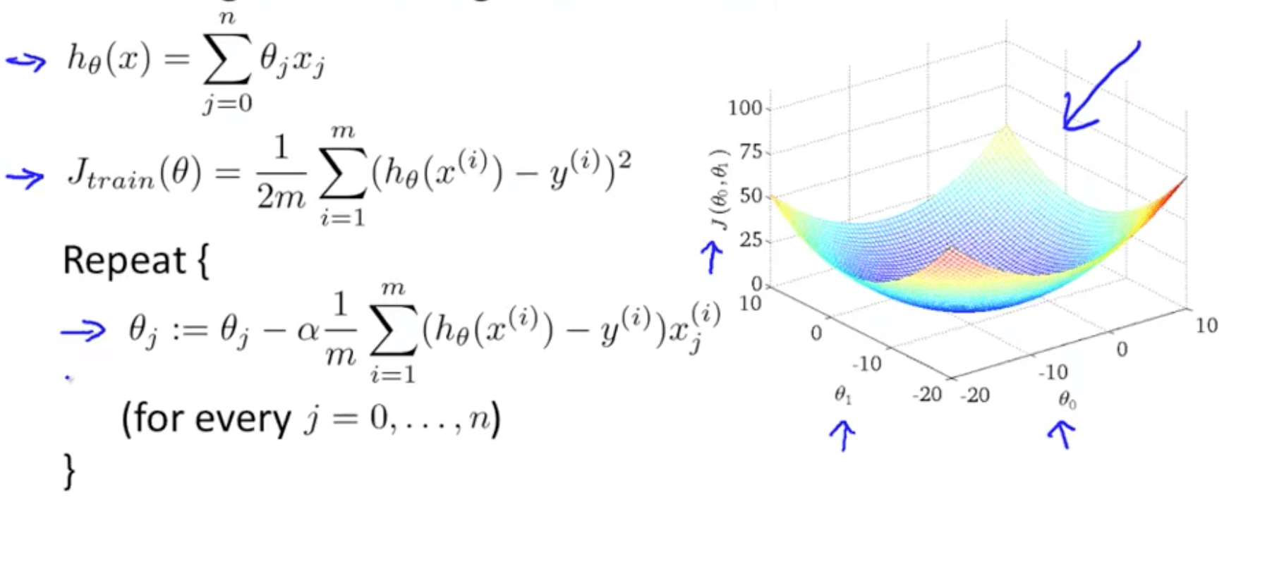
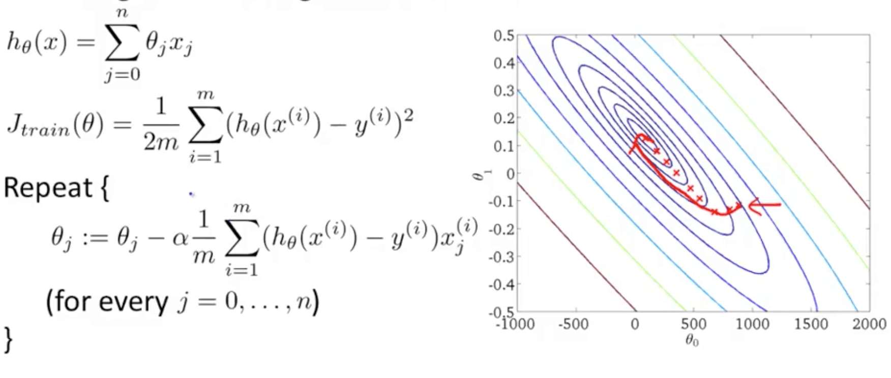
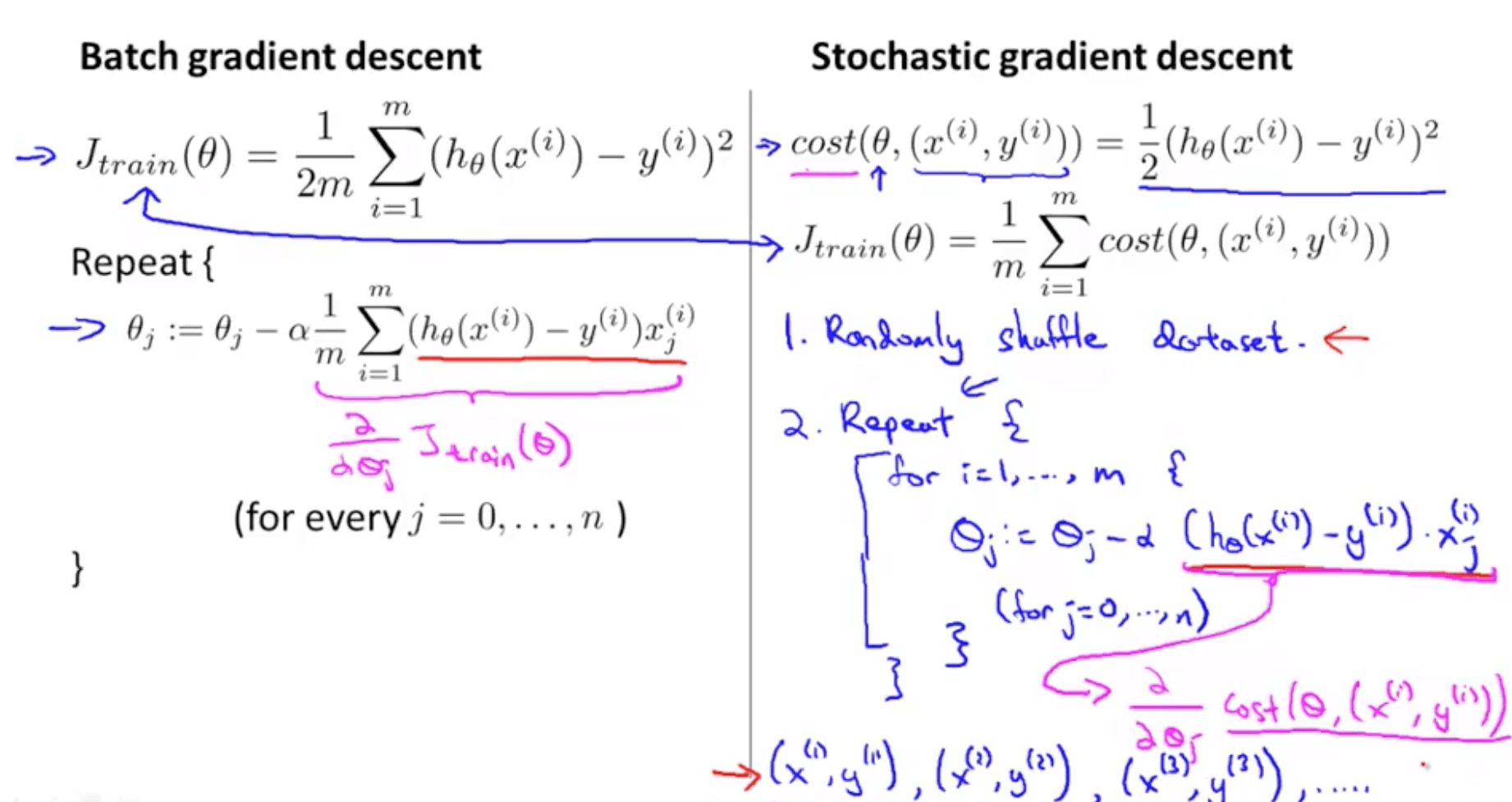
- Suppose we are training a linear regression model with gradient descent
- If m is really large, we have to sum across all the examples
- This is actually called batch gradient descent when you look at all the training examples
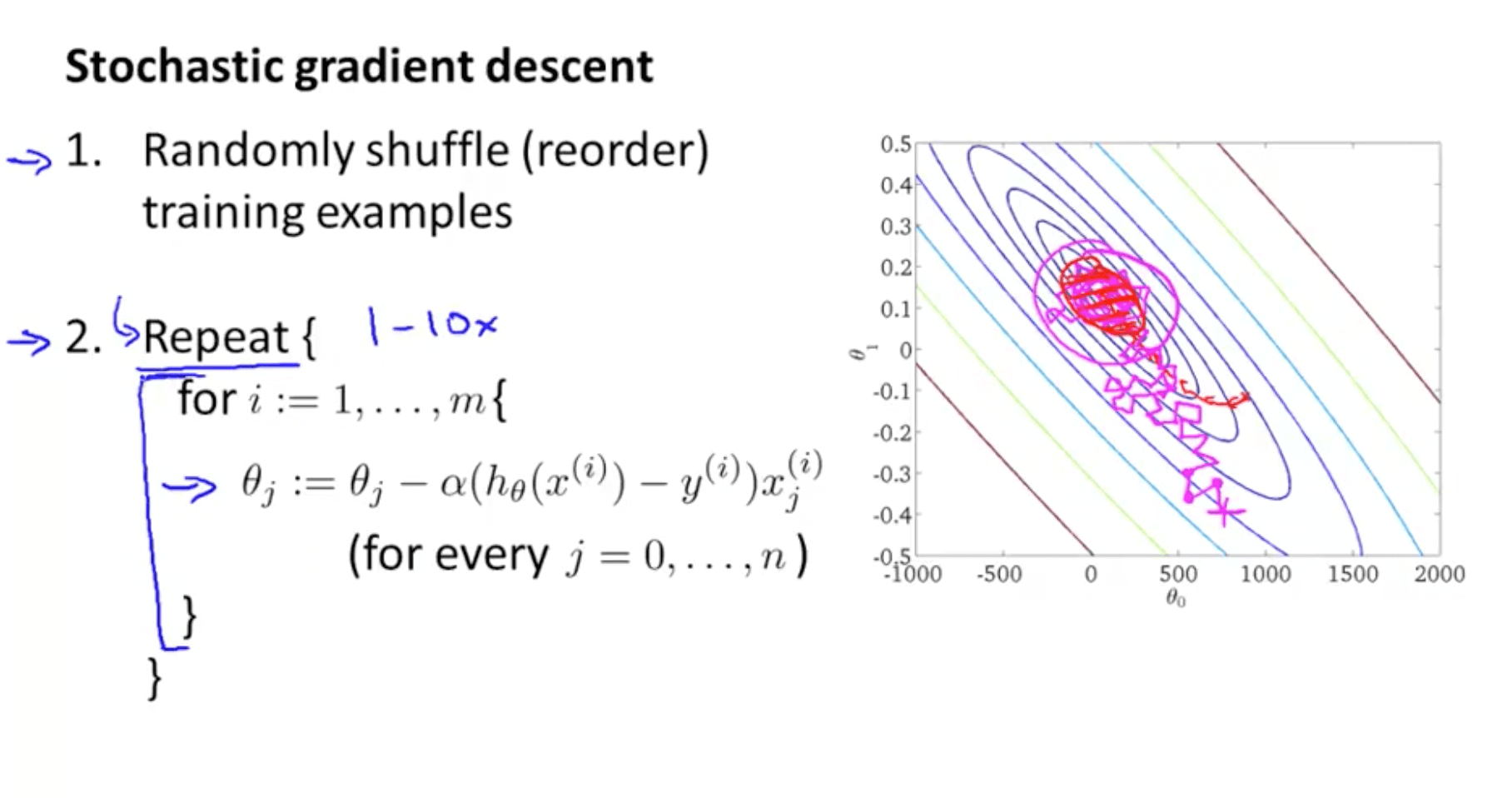
- We can use a stochastic gradient descent instead of a batch gradient descent
- Stochastic gradient descent (more efficient)
- Define cost of parameter θ with respect to x_i and y_i
- This measures how well the hypothesis is doing on a single training example (x_i, y_i)
- This algorithm will take the first training example and take a step (modify parameter) to fit the first example better until the end of the training set
- Difference
- Rather than waiting to take the parts of all the training examples (batch gradient descent), we look at a single training example and we are making progress towards moving to the global minimum
- Batch gradient descent (red path)
- Stochastic gradient descent (magenta path with a more random-looking path where it wonders around near the global minimum)
- In practice, so long the parameters are near the global minimum, it’s sufficient
- We can repeat the loop maybe 1 to 10 times
- It is possible even with 1 loop, where your m is large, you can have good parameters
- Your J_train (cost function) may not decrease with every iteration for stochastic gradient descent
- Define cost of parameter θ with respect to x_i and y_i
- Stochastic gradient descent (more efficient)
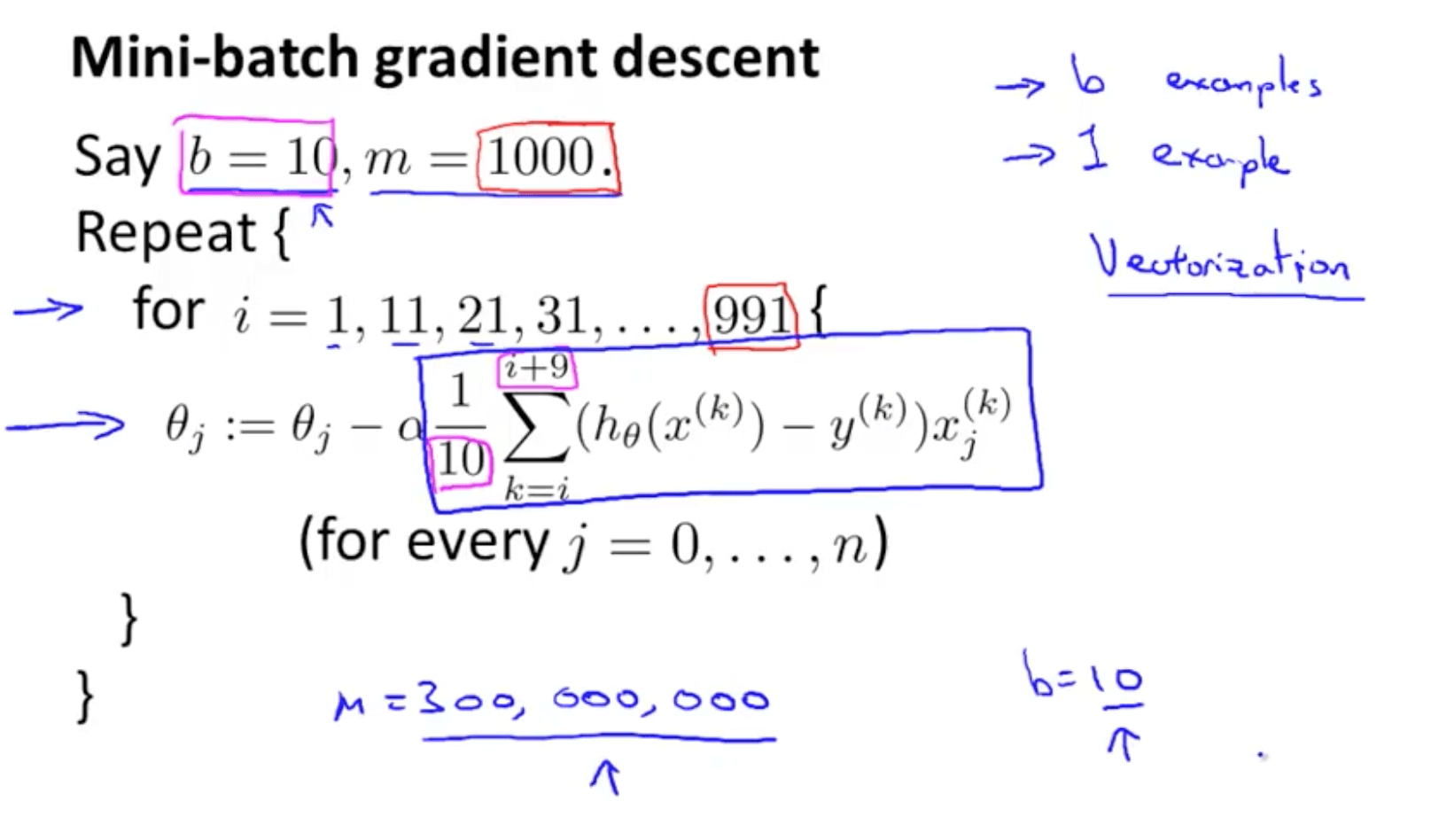
1c. Mini-Batch Gradient Descent
- This may some times be faster than stochastic gradient descent
- Difference
- Batch gradient descent
- Use all m examples in each iteration
- Stochastic gradient descent
- Use 1 example in each iteration
- Mini-batch gradient descent
- Use b examples in each iteration
- b = mini-batch size
- b = 10 examples
- Batch gradient descent
- Mini-batch gradient descent algorithm
- After looking at the 10 training examples, we start making progress in modifying the parameters
- Mini-batch gradient descent can outperform stochastic gradient descent if we use a vectorized implementation
- This algorithm is the same as batch gradient descent if b = m, where we iterate across all training examples
1d. Stochastic Gradient Descent Convergence
- Checking for convergence
- When you average over a smaller number of examples, there might be too much noise
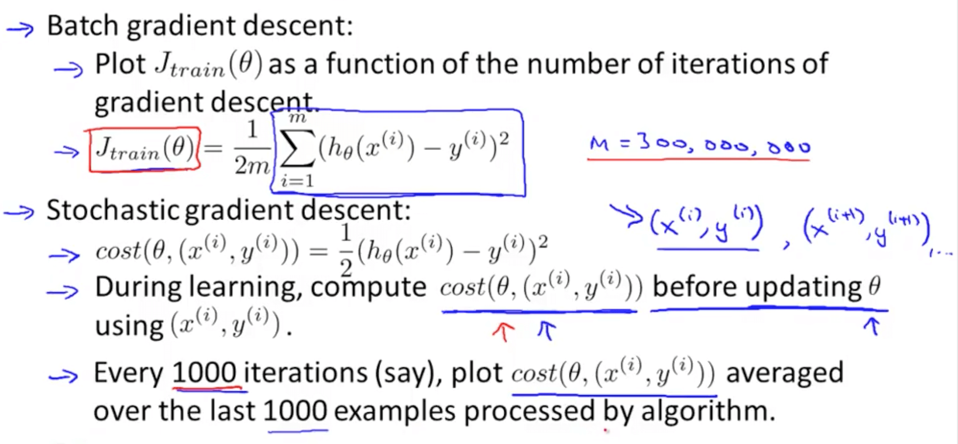
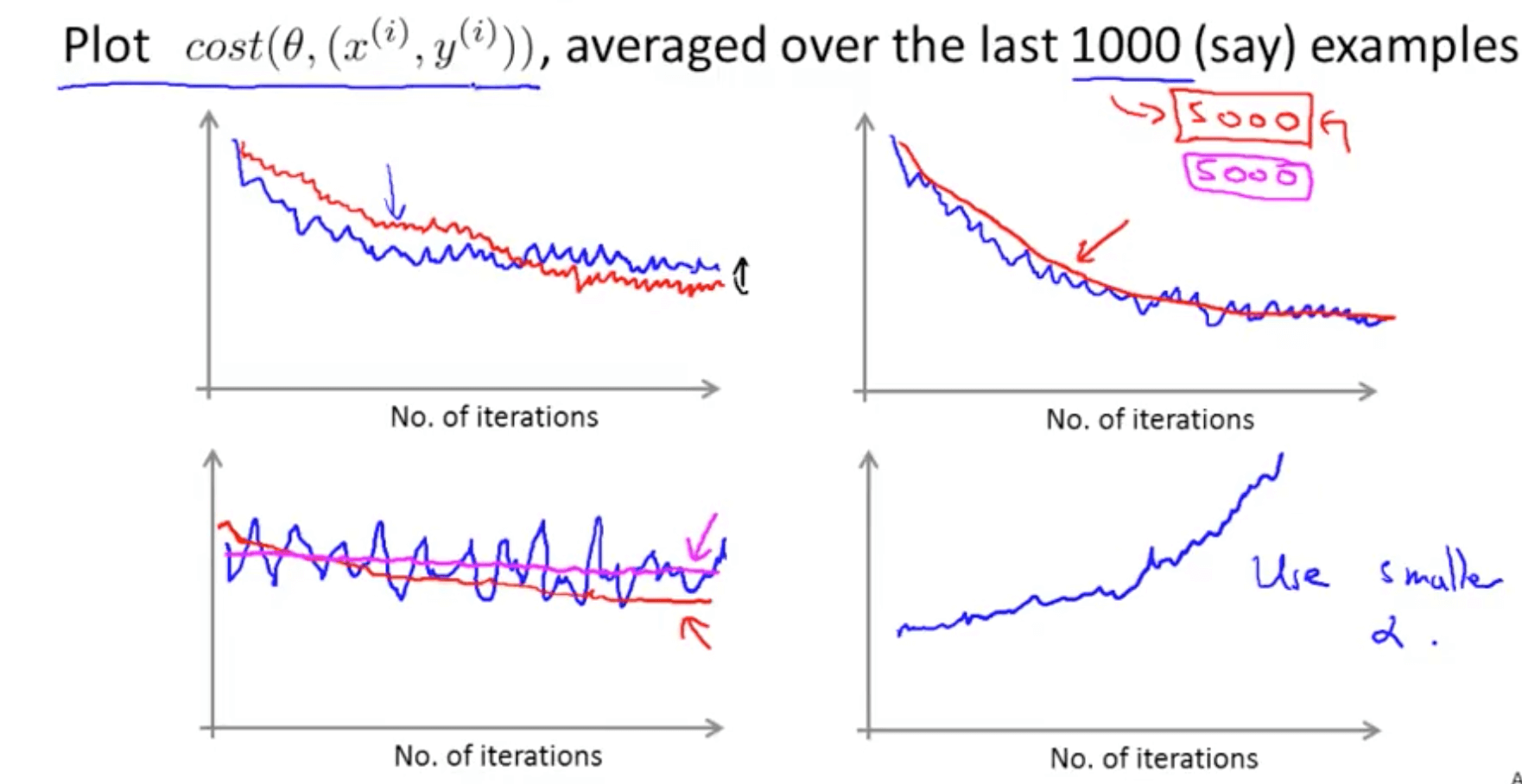
- When you average over a smaller number of examples, there might be too much noise
- Stochastic gradient descent learning rate issue
- Decrease learning rate to allow convergence for a slightly better hypothesis
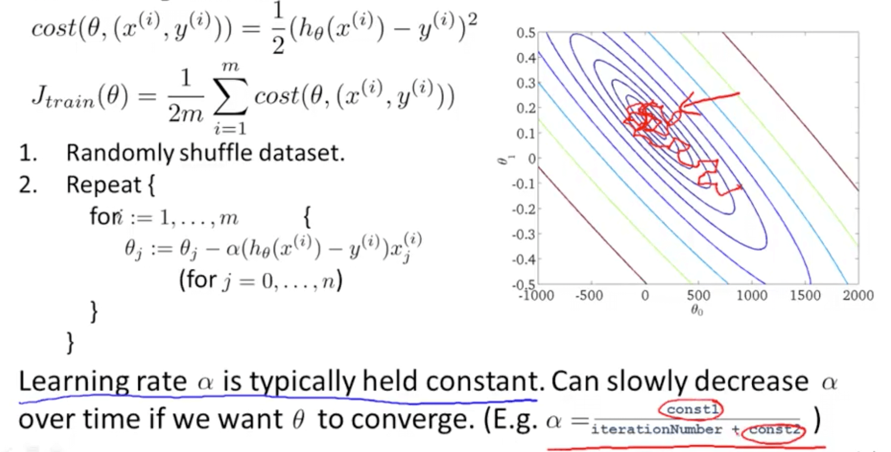
- Decrease learning rate to allow convergence for a slightly better hypothesis
2. Advanced Topics
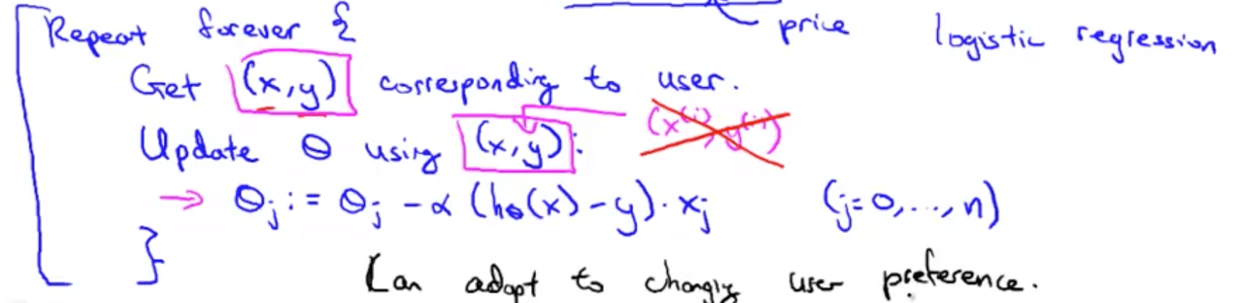
2a. Online Learning
- What is online learning?
- When we have a continuous stream of information and we want to learn from that
- We can use an online learning algorithm to optimize some decisions
- Example of online learning: learning whether to buy or not buy
- Shipping service website where user comes, specifies origin and destination, you offer to ship their package for some asking price, and users sometimes choose to use your shipping service (y = 1), sometimes not (y = 0)
- Features x captures properties of user, of origin/destination and asking price
-
We want to learn p(y = 1 x;θ) to optimize price - Probability of 1 given price and features
- We can use logistic regression or neural network
- Online learning algorithm
- If you have a large number of users, you can do this
- If you have a small number of users, you should save the data and train your parameters on your training data, not on a continuous stream of data
- This online algorithm can adapt to users’ preferences
- Example 2 of online learning: learning to search
- User searches for “Android phone 1080p camera”
- Have 100 phones in store with 10 results
- x = features of phone, how many words in user query match name of phone, how many words in query match description of phone
- y = 1 if user clicks on link
- y = 0 if otherwise
-
We want to learn p(y = 1 x;θ) to predict CTR - Use to show users’ 10 phones they’re most likely to click on
- Other examples
- Choosing special offers to show user
- Customized selection of news articles
- Product recommendation
2b. Map Reduce and Data Parallelism
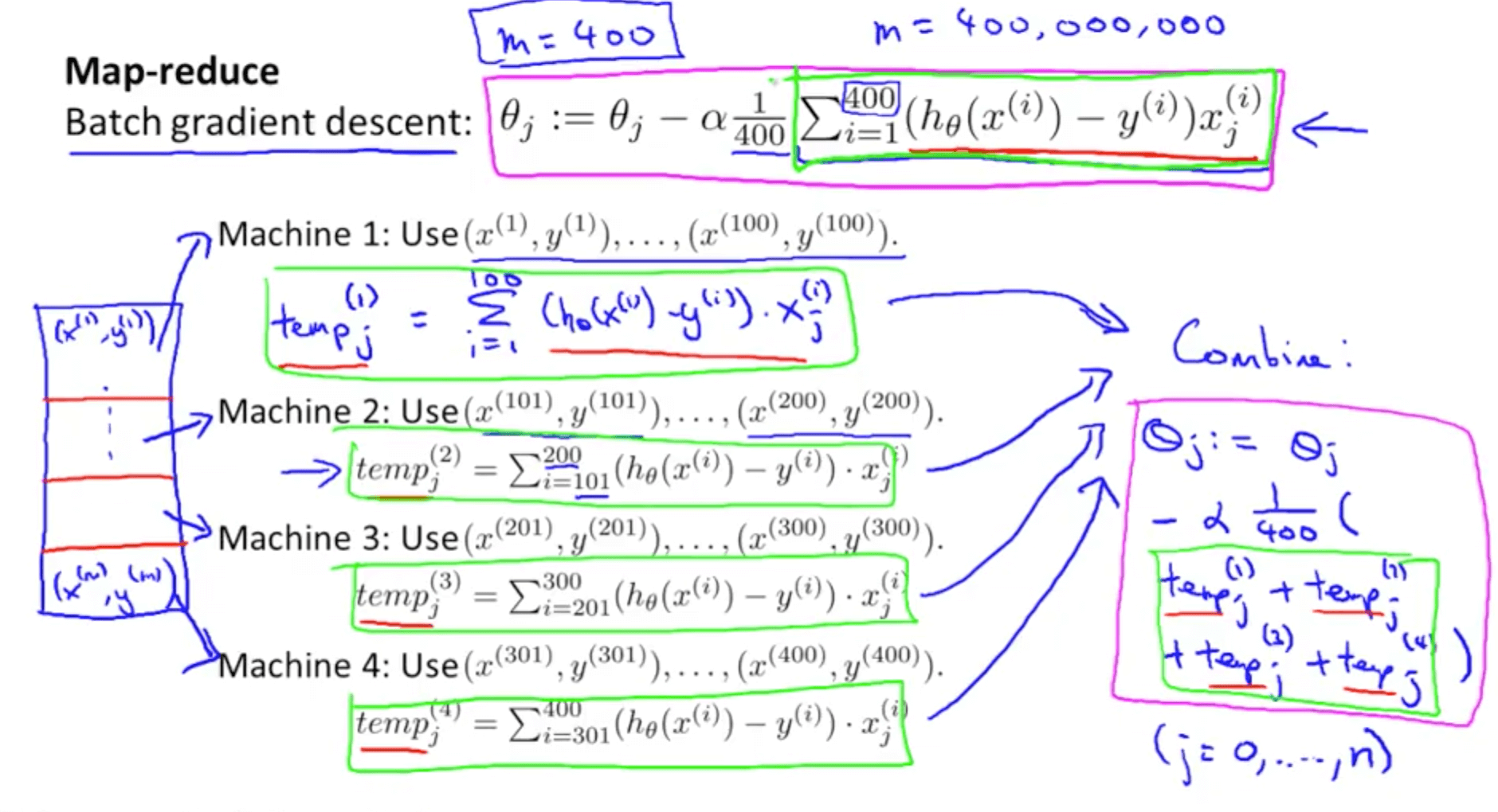
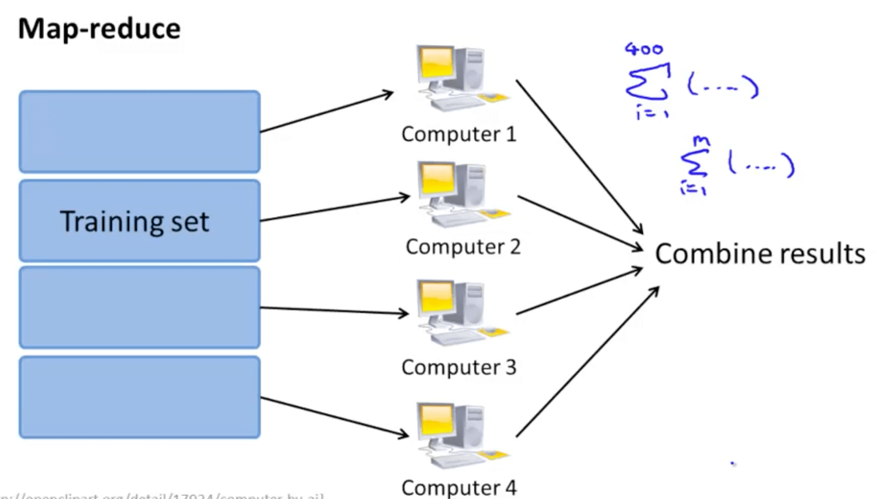
- Map reduce and linear regression
- This is an alternative to stochastic gradient descent and mini-batch gradient descent
- It is exactly equal to batch gradient descent but
- Split the training sets
- Split to 4 computers
- Combine results
- Many learning algorithms can be expressed as computing sums of functions over the training set
- Map reduce and logistic regression
- This can be done too as we can compute sums of fractions
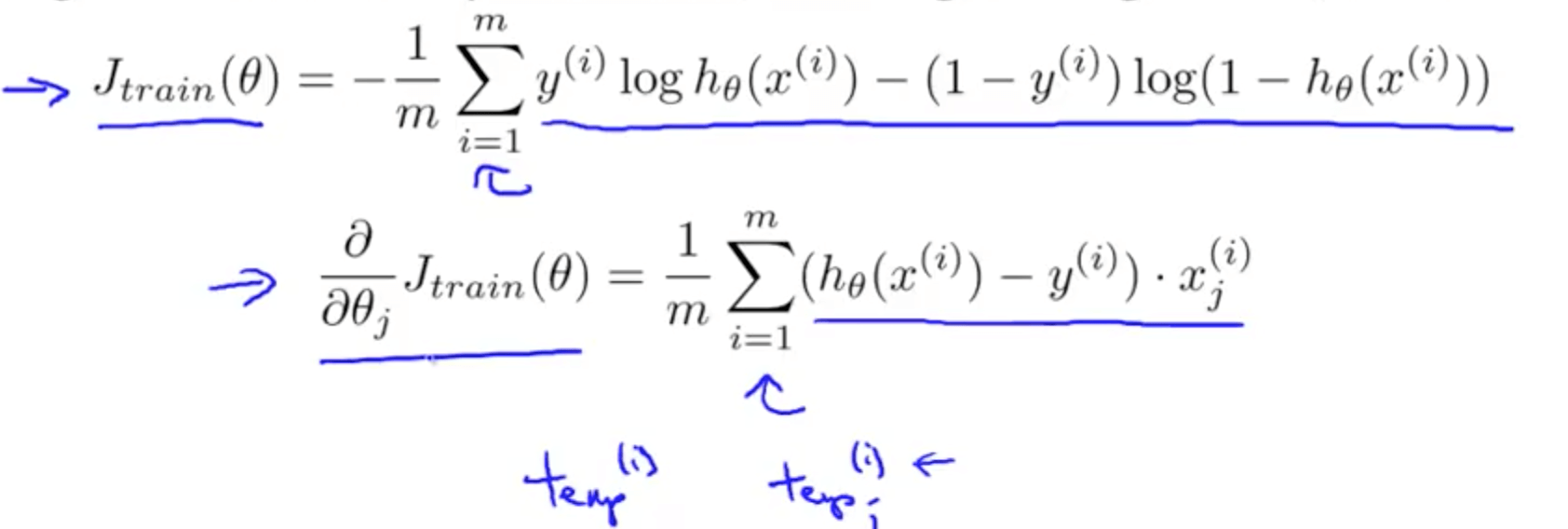
- This can be done too as we can compute sums of fractions
- Map reduce and neural network
- Suppose you want to apply map-reduce to train a neural network on 10 machines
- In each iteration, compute forward propagation and back propagation on 1/10 of the data to compute the derivative with respect to that 1/10 of the data
- Suppose you want to apply map-reduce to train a neural network on 10 machines
- Multi-core machines
- We can split training sets to different cores and then combine the results
- “Parallelizing” over multiple cores in the same machine makes network latency less of an issue
- There are some libraries to automatically “parallelize” by just implementing the usual vectorized implementation
- We can split training sets to different cores and then combine the results