Topics
- Evaluation procedure 1 - Train and test on the entire dataset
- a. Logistic regression
- b. KNN (k = 5)
- c. KNN (k = 1)
- d. Problems with training and testing on the same data
- Evaluation procedure 2 - Train/test split
- Making predictions on out-of-sample data
- Downsides of train/test split
- Resources
I would like to give full credits to the respective authors as these are my personal python notebooks taken from deep learning courses from Andrew Ng, Data School and Udemy :) This is a simple python notebook hosted generously through Github Pages that is on my main personal notes repository on https://github.com/ritchieng/ritchieng.github.io. They are meant for my personal review but I have open-source my repository of personal notes as a lot of people found it useful.
1. Evaluation procedure 1 - Train and test on the entire dataset
- Train the model on the entire dataset.
- Test the model on the same dataset, and evaluate how well we did by comparing the predicted response values with the true response values.
# read in the iris data
from sklearn.datasets import load_iris
iris = load_iris()

# create X (features) and y (response)
X = iris.data
y = iris.target
1a. Logistic regression
# import the class
from sklearn.linear_model import LogisticRegression

# instantiate the model (using the default parameters)
logreg = LogisticRegression()

# fit the model with data
logreg.fit(X, y)

# predict the response values for the observations in X
logreg.predict(X)
# store the predicted response values
y_pred = logreg.predict(X)

# check how many predictions were generated
len(y_pred)
Classification accuracy:
- Proportion of correct predictions
- Common evaluation metric for classification problems
# compute classification accuracy for the logistic regression model
from sklearn import metrics

print(metrics.accuracy_score(y, y_pred))
- Known as training accuracy when you train and test the model on the same data
- 96% of our predictions are correct
1b. KNN (K=5)
from sklearn.neighbors import KNeighborsClassifier
knn = KNeighborsClassifier(n_neighbors=5)
knn.fit(X, y)
y_pred = knn.predict(X)
print(metrics.accuracy_score(y, y_pred))
It seems, there is a higher accuracy here but there is a big issue of testing on your training data
1c. KNN (K=1)
knn = KNeighborsClassifier(n_neighbors=1)
knn.fit(X, y)
y_pred = knn.predict(X)
print(metrics.accuracy_score(y, y_pred))
- KNN model
- Pick a value for K.
- Search for the K observations in the training data that are "nearest" to the measurements of the unknown iris
- Use the most popular response value from the K nearest neighbors as the predicted response value for the unknown iris
- This would always have 100% accuracy, because we are testing on the exact same data, it would always make correct predictions
- KNN would search for one nearest observation and find that exact same observation
- KNN has memorized the training set
- Because we testing on the exact same data, it would always make the same prediction
1d. Problems with training and testing on the same data
- Goal is to estimate likely performance of a model on out-of-sample data
- But, maximizing training accuracy rewards overly complex models that won't necessarily generalize
- Unnecessarily complex models overfit the training data
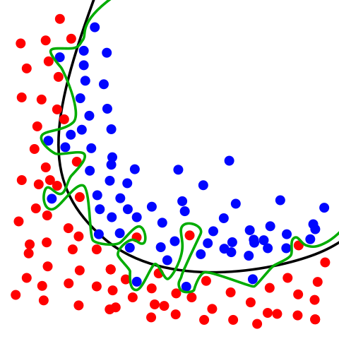
Image Credit: Overfitting by Chabacano. Licensed under GFDL via Wikimedia Commons.
- Green line (decision boundary): overfit
- Your accuracy would be high but may not generalize well for future observations
- Your accuracy is high because it is perfect in classifying your training data but not out-of-sample data
- Black line (decision boundary): just right
- Good for generalizing for future observations
- Hence we need to solve this issue using a train/test split that will be explained below
2. Evaluation procedure 2 - Train/test split
- Split the dataset into two pieces: a training set and a testing set.
- Train the model on the training set.
- Test the model on the testing set, and evaluate how well we did.
# print the shapes of X and y
# X is our features matrix with 150 x 4 dimension
print(X.shape)
# y is our response vector with 150 x 1 dimension
print(y.shape)
# STEP 1: split X and y into training and testing sets
from sklearn.cross_validation import train_test_split
X_train, X_test, y_train, y_test = train_test_split(X, y, test_size=0.4, random_state=4)
- test_size=0.4
- 40% of observations to test set
- 60% of observations to training set
- data is randomly assigned unless you use random_state hyperparameter
- If you use random_state=4
- Your data will be split exactly the same way
- If you use random_state=4
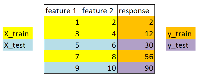
What did this accomplish?
- Model can be trained and tested on different data
- Response values are known for the testing set, and thus predictions can be evaluated
- Testing accuracy is a better estimate than training accuracy of out-of-sample performance
# print the shapes of the new X objects
print(X_train.shape)
print(X_test.shape)
# print the shapes of the new y objects
print(y_train.shape)
print(y_test.shape)
# STEP 2: train the model on the training set
logreg = LogisticRegression()
logreg.fit(X_train, y_train)
# STEP 3: make predictions on the testing set
y_pred = logreg.predict(X_test)

# compare actual response values (y_test) with predicted response values (y_pred)
print(metrics.accuracy_score(y_test, y_pred))
Repeat for KNN with K=5:
knn = KNeighborsClassifier(n_neighbors=5)
knn.fit(X_train, y_train)
y_pred = knn.predict(X_test)
print(metrics.accuracy_score(y_test, y_pred))
Repeat for KNN with K=1:
knn = KNeighborsClassifier(n_neighbors=5)
knn.fit(X_train, y_train)
y_pred = knn.predict(X_test)
print(metrics.accuracy_score(y_test, y_pred))
Can we locate an even better value for K?
# try K=1 through K=25 and record testing accuracy
k_range = range(1, 26)

# We can create Python dictionary using [] or dict()
scores = []

# We use a loop through the range 1 to 26
# We append the scores in the dictionary
for k in k_range:
    knn = KNeighborsClassifier(n_neighbors=k)
    knn.fit(X_train, y_train)
    y_pred = knn.predict(X_test)
    scores.append(metrics.accuracy_score(y_test, y_pred))

print(scores)
# import Matplotlib (scientific plotting library)
import matplotlib.pyplot as plt

# allow plots to appear within the notebook
%matplotlib inline

# plot the relationship between K and testing accuracy
# plt.plot(x_axis, y_axis)
plt.plot(k_range, scores)
plt.xlabel('Value of K for KNN')
plt.ylabel('Testing Accuracy')

- Training accuracy rises as model complexity increases
- Testing accuracy penalizes models that are too complex or not complex enough
- For KNN models, complexity is determined by the value of K (lower value = more complex)
3. Making predictions on out-of-sample data
# instantiate the model with the best known parameters
knn = KNeighborsClassifier(n_neighbors=11)

# train the model with X and y (not X_train and y_train)
knn.fit(X, y)

# make a prediction for an out-of-sample observation
knn.predict([3, 5, 4, 2])
4. Downsides of train/test split
- Provides a high-variance estimate of out-of-sample accuracy
- K-fold cross-validation overcomes this limitation
- But, train/test split is still useful because of its flexibility and speed
5. Resources
- Quora: What is an intuitive explanation of overfitting?
- Video: Estimating prediction error (12 minutes, starting at 2:34) by Hastie and Tibshirani
- Understanding the Bias-Variance Tradeoff
- Guiding questions when reading this article
- Video: Visualizing bias and variance (15 minutes) by Abu-Mostafa