Solve MDPs' equations and understand the intuition behind it leading to reinforcement learning.
Markov Decision Processes
Differences in Learning
- Supervised learning: y = f(x)
- Given x-y pairs
- Learn function f(x)
- Function approximation
- Unsupervised learning: f(x)
- Given x's
- Learn the function f(x)
- Clustering description
- Reinforcement learning:
- Given x's and z's
- Learn function f(x)
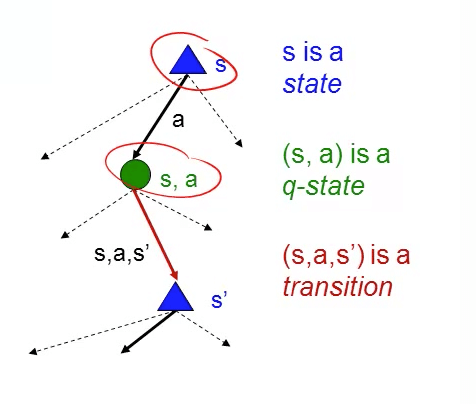
Markov Decision Processes
- States: S
- They are kind of like positions on a map if you are navigating to an end point
- Model (Transition Function): T(s, a, s') ~ P(s' | s, a)
- The model is like a set of rules for a game (physics of the world).
- s: state
- a: action
- s': another state
- Probability of s' given s and a
- Simple: if you're in a deterministic world, if you go straight (a) from the toilet (s), you would go straight (s') with a probability of 1.
- Slightly complex: can be that you have a probability of only 0.8 if you choose to go up, you may go right with a probability of 0.2.
- Your potential state (s') is only dependent on your current state (s) if not you will have more s-es.
- This is a Markovian property where only the present matters.
- Also, given the present state, the future and the past are independent.
- Actions: A(s), A
- They are things you can do such as going up, down, left and right if you are navigating through a box grid.
- They can be other kinds of actions too, depending on your scenario.
- Reward: R(s), R(s, a), R(s, a, s')
- Scalar value for being in a state.
- Position 1, you'll have 100 points.
- Position 2, you'll have -10 points.
- R(s): reward for being in a state
- R(s, a): reward for being in a state and taking an action
- R(s, a, s'): reward for being in a state, taking an action and ending up in the other state
- They are mathematically equivalent.
- Scalar value for being in a state.
- Policy: π(s) → a
- This is basically the solution: what action to take in any particular state.
- It takes in a state, s, and it tells you the action, a, to take.
- π* optimizes the amount the reward at any given point in time.
- Here we have (s, a, r) triplets.
- We need to find the optimal action
- Given what we know above
- π*: function f(x)
- r: z
- s: x
- a: y
- Here we have (s, a, r) triplets.
- Visualization
Rewards (Domain Knowledge)
- Delayed rewards
- You won't know what your immediate action would lead to down the road.
- Example in chess
- You did many moves
- Then you have your final reward where you did well or badly
- You could have done well at the start then worst at the end.
- You could have done badly at the start then better at the end.
- Example in chess
- You won't know what your immediate action would lead to down the road.
- Example
- R(s) = -0.01
- Reward for every state except for the 2 absorbing states is -0.01.
- s_good = +1
- s_bad = -0.01
- Each action you take, you get punished.
- You are encouraged to end the game soon.
- Minor changes to your reward function matters a lot.
- If you have a huge negative reward, you will be in a hurry.
- If you have a small negative reward, you may not be in a hurry to reach the end.
- R(s) = -0.01
Sequence of rewards: assumptions
- Stationary preferences
- [a1, a2, ...] > [b1, b2, ...]
- [r, a1, a2, ...] > [r, b1, b2, ...]
- You'll do the same action regardless of time.
- Inifinite horizons
- The game does not end until we reach the absorbing state.
- If we do not have an inifinite time, and a short amount of time, we may want to rush through to get a positive reward.
- Policy with finite horizon: π(s, t) → a
- This would terminate after t
- Gives non-stationary polices where states' utilities changes with time.
- Policy with finite horizon: π(s, t) → a
- Utility of sequences
- We will be adding rewards using discounted sums.
- $$ U(S_0 S_1 ...) = \sum_{i=0}^∞ γ^tR(S_t) = \frac {R_{max}}{1 - γ}$$
- $$ 0 ≤ γ < 1 $$
- If we do not multiply by gamma, all the rewards would sum to infinity.
- When we multiply by gamma, we get a geometric series that allows us to multiply an infinite number of rewards to get a finite number.
- Also, the discount factor is multiplied because sooner rewards probably have higher utility than later rewards.
- Things in the future are discounted so much they become negligible. Hence, we reach a finite number for our utility.
- Absorbing state
- Guarantee that for every policy, a terminal state will eventually be reached.
Optimal Policy
- $$ π^* = argmax_π \ E \ [ \sum_{i=0}^∞γ^tR(s_t) \ | \ π ] $$
- Expectation because it is non-deterministic
- π*: optimal policy
- $$ U^π(s) = E \ [ \sum_{i=0}^∞γ^tR(s_t) \ | \ π, \ s_0 = s ] $$
- Utility of a particular state depends on the policy we are taking π
- Utility is what we expect to see from then.
- This is not equal to the reward, R(s) for being in that state that is immediate.
- If you look at going to university, there's an immediate negative reward, say paying for school fees. But in the long-run you may have higher salary which is similar to U(s), a form of delayed reward.
- Utility, U(s) gives us a long-term view.
- $$ π^*(s) = argmax_a \sum_{s'}T(s, a, s') U(s') $$
- This is the optimal action to take at a state.
- For every state, returns an action that maximizes my expected utility.
- $$ U(s) = R(s) + γ \ argmax_a \sum_{s'}T(s, a, s') U(s') $$
- True utility of that state U(s): R(S) + expected utility
- Belman equation.
- Reward of that state plus the discount of all the reward from then on.
- T(s, a, s'): model.
- U(s'): utility of another state.
- Reward of that state plus the discount of all the reward from then on.
- n equations: since we've n number of states.
- n unknowns: U(s') since we've n number of states.
Finding Policies: Value Iteration
- We start with arbitrary utilities
- For example, 0.
- Update utilities based on neighbours (all the states it can reach).
- $$ \hat {U}_{t+1}(s) = R(s) + γ \ argmax_a \sum_{s'}T(s, a, s') \ \hat {U}_t(s') $$
- Bellman update equation.
- Repeat until convergence
Finding Policies: Policy Iteration
- Start with by guessing
- $$π_0$$
- Evaluate
- Given
- $$π_t$$
- Calculate
- $$u_t = u^{π_t}$$
- Given
- Improve: maximizing expected utility
- $$ π_{t+1} = argmax_a \sum_{s'}T(s, a, s') \ U_t(s') $$
- $$ U_t(s) = R(s) + γ \ \sum_{s'}T(s, a, s') U_t(s') $$