Getting started with the famous Iris dataset
Topics
- About Iris dataset
- Display Iris dataset
- Supervised learning on Iris dataset
- Loading the Iris dataset into scikit-learn
- Machine learning terminology
- Exploring the Iris dataset
- Requirements for working with datasets in scikit-learn
- Additional resources
This tutorial is derived from Data School's Machine Learning with scikit-learn tutorial. I added my own notes so anyone, including myself, can refer to this tutorial without watching the videos.
1. About Iris dataset
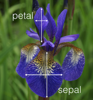
- The iris dataset contains the following data
- 50 samples of 3 different species of iris (150 samples total)
- Measurements: sepal length, sepal width, petal length, petal width
- The format for the data: (sepal length, sepal width, petal length, petal width)
2. Display Iris Dataset
In [1]:
# Display HTML using IPython.display module
# You can display any other HTML using this module too
# Just replace the link with your desired HTML page
from IPython.display import HTML
HTML('<iframe src=http://archive.ics.uci.edu/ml/machine-learning-databases/iris/iris.data width=300 height=200></iframe>')
Out[1]:
3. Supervised learning on the iris dataset
- Framed as a supervised learning problem
- Predict the species of an iris using the measurements
- Famous dataset for machine learning because prediction is easy
- Learn more about the iris dataset: UCI Machine Learning Repository
4. Loading the iris dataset into scikit-learn
In [2]:
# import load_iris function from datasets module
# convention is to import modules instead of sklearn as a whole
from sklearn.datasets import load_iris
In [3]:
# save "bunch" object containing iris dataset and its attributes
# the data type is "bunch"
iris = load_iris()
type(iris)
Out[3]:
In [5]:
# print the iris data
# same data as shown previously
# each row represents each sample
# each column represents the features
print(iris.data)
5. Machine learning terminology
- Each row is an observation (also known as: sample, example, instance, record)
- Each column is a feature (also known as: predictor, attribute, independent variable, input, regressor, covariate)
6. Exploring the iris dataset
In [ ]:
# print the names of the four features
print iris.feature_names
In [ ]:
# print integers representing the species of each observation
# 0, 1, and 2 represent different species
print iris.target
In [ ]:
# print the encoding scheme for species: 0 = setosa, 1 = versicolor, 2 = virginica
print iris.target_names
- Each value we are predicting is the response (also known as: target, outcome, label, dependent variable)
- Classification is supervised learning in which the response is categorical
- "0": setosa
- "1": versicolor
- "2": virginica
- Regression is supervised learning in which the response is ordered and continuous
- any number (continuous)
7. Requirements for working with data in scikit-learn
- Features and response are separate objects
- In this case, data and target are separate
- Features and response should be numeric
- In this case, features and response are numeric with the matrix dimension of 150 x 4
- Features and response should be NumPy arrays
- The iris dataset contains NumPy arrays already
- For other dataset, by loading them into NumPy
- Features and response should have specific shapes
- 150 x 4 for whole dataset
- 150 x 1 for examples
- 4 x 1 for features
- you can convert the matrix accordingly using np.tile(a, [4, 1]), where a is the matrix and [4, 1] is the intended matrix dimensionality
In [6]:
# check the types of the features and response
print(type(iris.data))
print(type(iris.target))
In [8]:
# check the shape of the features (first dimension = number of observations, second dimensions = number of features)
print(iris.data.shape)
In [7]:
# check the shape of the response (single dimension matching the number of observations)
print(iris.target.shape)
In [ ]:
# store feature matrix in "X"
X = iris.data

# store response vector in "y"
y = iris.target
8. Resources
- scikit-learn documentation: Dataset loading utilities
- Jake VanderPlas: Fast Numerical Computing with NumPy (slides, video)
- Scott Shell: An Introduction to NumPy (PDF)